
These are the lecture notes for FAU’s YouTube Lecture “Pattern Recognition“. This is a full transcript of the lecture video & matching slides. We hope, you enjoy this as much as the videos. Of course, this transcript was created with deep learning techniques largely automatically and only minor manual modifications were performed. Try it yourself! If you spot mistakes, please let us know!
Welcome back to Pattern Recognition! Today, we want to look a little more into the modeling of decision boundaries. In particular, we are interested in what is happening with other distributions. We are also interested in what is happening if we have equal dispersion or standard deviations in different distributions.
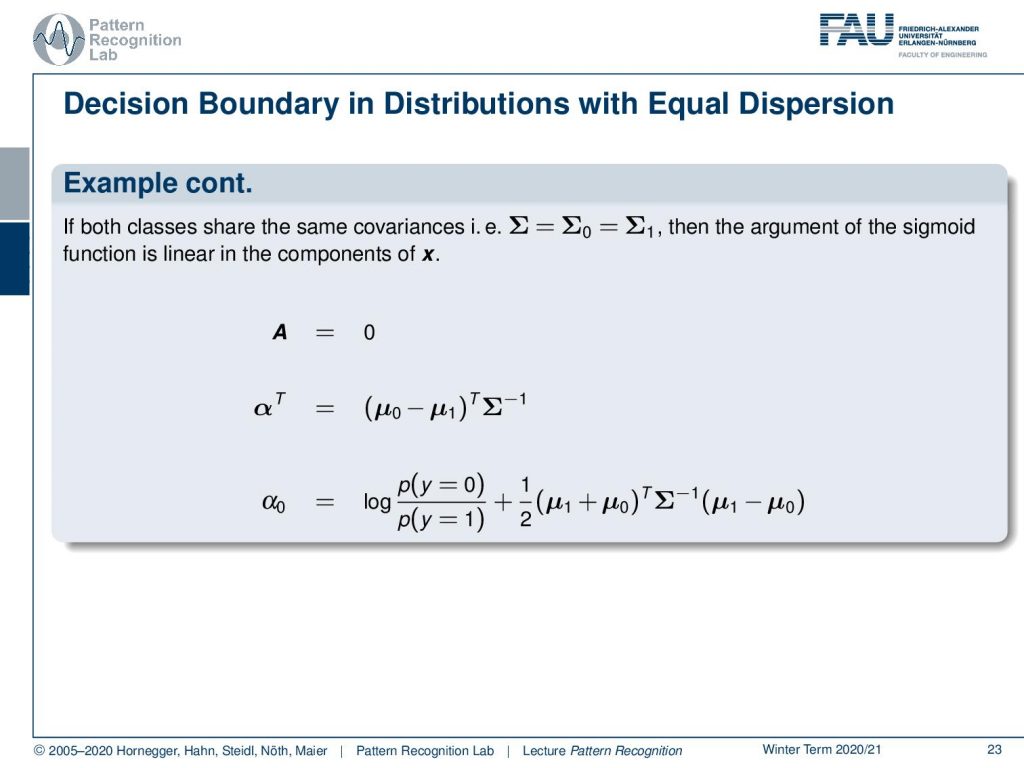
Now we want to look into a special case. The special case with the Gaussian here is that we have a covariance matrix that is identical for both classes. And if we do so, we can see that the formulation that we found earlier in the previous video collapses in particular to a simplification of the matrix A. So matrix A was the quadratic part, and this is simply a zero matrix now. This means essentially that the entire quadratic part cancels out because we are simply multiplying the one matrix with the inverse of the other matrix. They’re identical, so they simply turn out to be zero. The nice thing here is that we can already see from the formulation that we find here that we essentially have a line that is separating now those two distributions. And the line is essentially given by the difference between the two means and it’s weighted by the inverse covariance matrix. Of course, there is an offset and the offset is mainly dependent on the prior probability for the two classes. This is weighted then by the difference of the two means multiplied by the inverse covariance matrix.
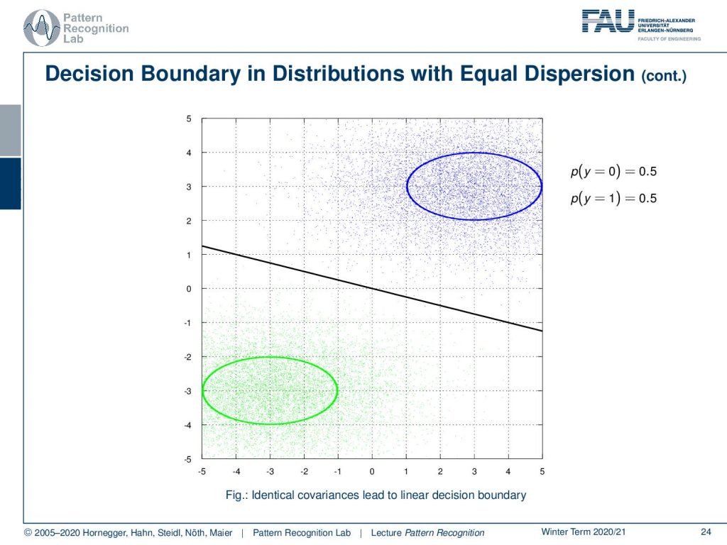
Well, if we look at this example here, you can already see these are now two Gaussians. Those two Gaussians have the same prior, and they are distributed with the same covariance matrix. And if we have this case, our decision boundary collapses to a line. This is simply the line as shown here. Again, if we would play with the priors, the line would move back and forth because this is altering the offset between the two classes.
So if the conditionals are Gaussians and share the same covariance, the exponential function is affine in x. This then results in a line as a decision boundary. The nice thing about this observation is that this result is also true for a more general function of probability density functions. So it’s not just limited to Gaussians. We do express this as Equal Dispersion.
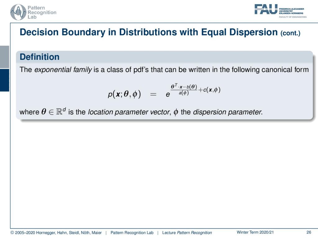
Generally, there is the exponential family of probability density functions and they can be written in the following canonical form. So this is some eᶿ, which is essentially the location parameter vector. This is multiplied as an inner product with x. Then there is some function b(θ), and this is divided by the dispersion parameter. Then we still add some c(x) and the dispersion which is essentially then able to add some additional bias turn on top here. So you see that this canonical form is implying several functions b, c, and a. We’re not defining the functions here right now. But if we use this kind of parametrization, we can then see quite a few probability density functions can be expressed in the following way.
So let’s look into the exponential family! Of course, we find the Gaussian probability density function here. You’ve already seen that there are different ways of formulating the Gaussian. Here we have all diagonal covariance matrices, and obviously, there are also non-diagonal covariance matrices. This then results in this rotation here as you can see. So this is a very typical function that we’re using to model the probability densities.
Then, we also have the exponential probability density function. You can see here that generally, functions that can be expressed as λ times e to the power of minus λ x fall into this category. This kind of function is very interesting because these are exponential decays. So these are probabilities for observing decays and are very commonly used for example in radioactivity. The functions generally follow this kind of format. But this is also true for any kind of exponential decay. By the way, also beer foam follows this decay rule. So you can see if we vary the parameter we can find different kinds of decay functions.
Well, not just the exponential probability density function follows the exponential family. Also, the binomial probability mass function, which is given here as n choose k p ᵏ (1-p) ⁿ⁻ᵏ. And you see, these are repeated experiments, so for example the coin toss that we talked about earlier. So if we have the classical Bernoulli experiments or Multi-nulli experiments, they will follow very similar probability mass functions. And here you see different instances of the binomial probability mass function.
Also, the Poisson probability mass function follows this exponential family. So here you see the Poisson probability mass function. We see different observations here. This is also a very important observation because this kind of probability mass function is highly relevant, in particular for Poisson processes. And if you have been working with, for example, particle physics, x-rays, photon counts, and photon interaction you see that the Poisson probability mass function is essentially modeling x-ray generation.
Also noteworthy is the Hypergeometric probability mass function. With this one, you can describe essentially earn experiments where you take out certain samples without replacement. So this kind of function can describe probability experiments that are not using replacement. And here are some examples. You see that this equal dispersion property is actually a quite general one. It holds for quite a few probability mass or probability density functions.
So, if all class conditional densities are members of the same exponential family of probability density functions with equal dispersion, the decision boundary f(x=0) is linear in the components of x. That’s actually a pretty cool observation!
So what did we learn in the last couple of videos? Posteriors can be rewritten in terms of a logistic function. We can give the decision boundary F(x) and write it down with the posterior right away. We can also find the decision boundary for normally distributed feature vectors, and we’ve seen that this is always a quadratic function. And if Gaussians share the same covariances, the decision boundary is always a linear function. This actually also holds for other distributions. So actually a pretty interesting observation.

Well, this already brings us to the end. In the next video, we want to look a bit more into the logistic function, and in particular, we want to look into ideas on how to lift linear decision boundaries to more general applicability.
So thank you very much for listening and I’m looking forward to seeing you in the next video. Bye-bye!
If you liked this post, you can find more essays here, more educational material on Machine Learning here, or have a look at our Deep Learning Lecture. I would also appreciate a follow on YouTube, Twitter, Facebook, or LinkedIn in case you want to be informed about more essays, videos, and research in the future. This article is released under the Creative Commons 4.0 Attribution License and can be reprinted and modified if referenced. If you are interested in generating transcripts from video lectures try AutoBlog.
References
T. Hastie, R. Tibshirani, and J. Friedman: The Elements of Statistical Learning – Data Mining, Inference, and Prediction, 2nd edition, Springer, New York, 2009.
David W. Hosmer, Stanley Lemeshow: Applied Logistic Regression, 2nd Edition, John Wiley & Sons, Hoboken, 2000.