Lecture Notes in Pattern Recognition: Episode 38 – Adaboost & Exponential Loss

These are the lecture notes for FAU’s YouTube Lecture “Pattern Recognition“. This is a full transcript of the lecture video & matching slides. We hope, you enjoy this as much as the videos. Of course, this transcript was created with deep learning techniques largely automatically and only minor manual modifications were performed. Try it yourself! If you spot mistakes, please let us know!

Welcome back to Pattern Recognition. Today we want to continue looking into AdaBoost and in particular, we want to see the relation between AdaBoost and the exponential loss.

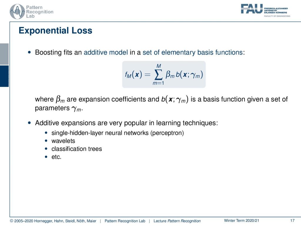
Boosting fits an additive model in a set of elementary basis functions. So the results of boosting are essentially created by expansion the coefficients β and some b, which is a basis function given a set of parameters γ. Additive expansion methods are very popular in learning techniques, you can see that very similar things are already applied in single hidden layer neural networks building on the perceptron in wavelets, classification trees and so on.

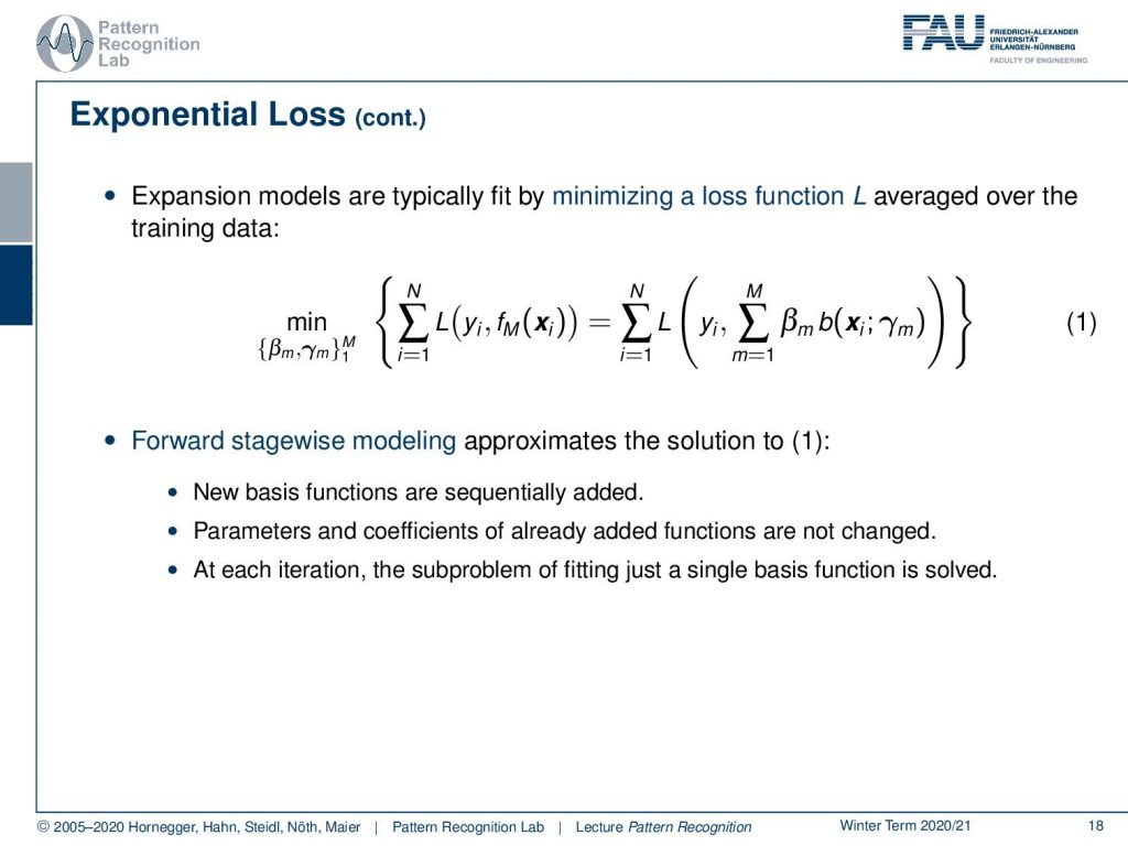
The expansion models are typically fit by minimizing a loss function L that is averaged over the training data. You essentially can write this as L over the entire training data, and then you can plug in our definition. And you see that we have this additive model that is essentially given by our function f_m. So the forward stagewise modelling approximates the solution to one. The new basis functions are sequentially added parameters. Coefficients of already added functions are not changed and at each iteration, only a subproblem of fitting, just a single basis function, is solved.

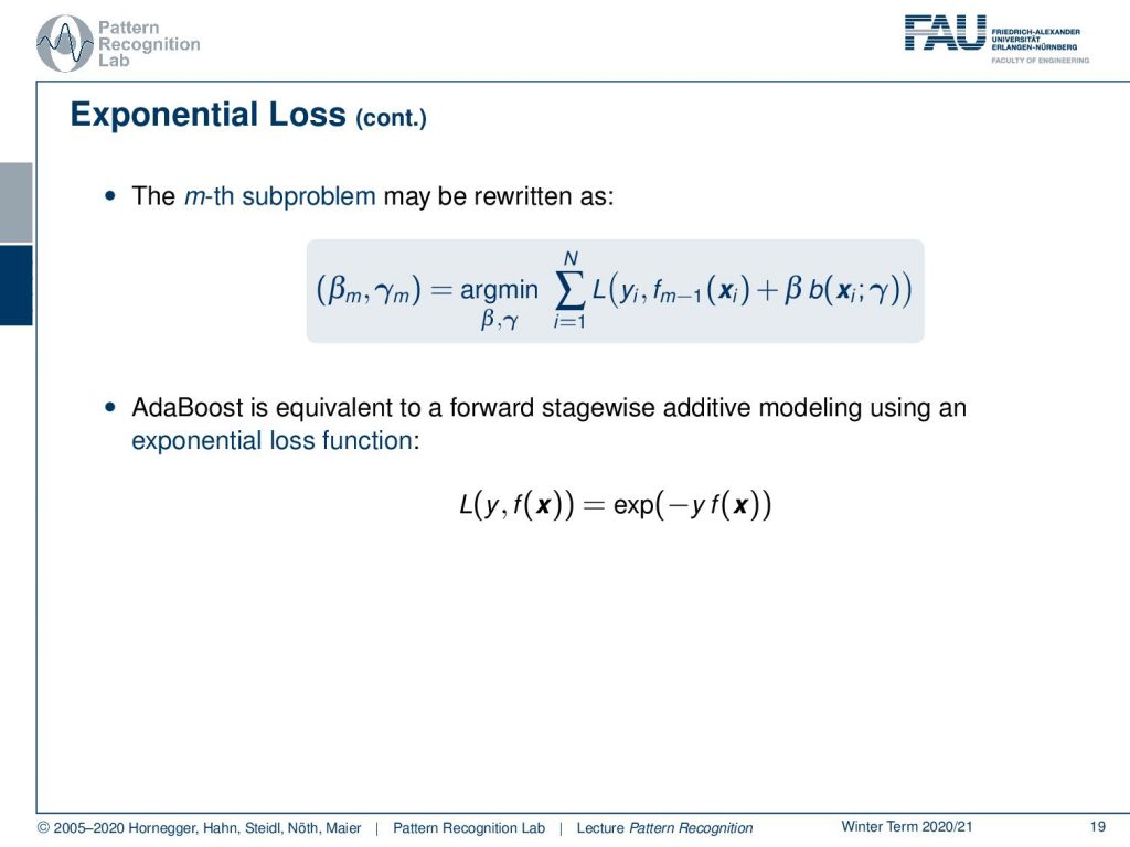
We can express now the m-th subproblem in the following way: We essentially have the loss of the (m – 1)-th solution plus β and the current estimate. We’re minimising over γ and β. Now Adaboost can be shown to be equivalent to forward stagewise additive modelling using an exponential loss function. So if our loss function equals to the exponent of minus y times f(x) we are essentially constructing the Adaboost loss.

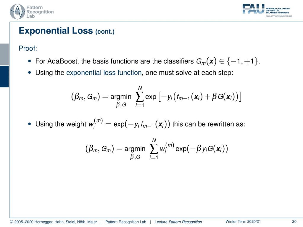
Let’s prove this. For AdaBoost, the basis functions are the classifiers G_m, and they produce the output of either – 1 or + 1. Using the exponential loss function, we now must solve at every step that we essentially minimise over β and G the sum over the exponential loss. If we now introduce a weight that we introduce here as w_i and we set it to the exponent of minus y times f_m-1(x_i). We can we rewrite this as a minimization of a weighted sum of exponential functions.

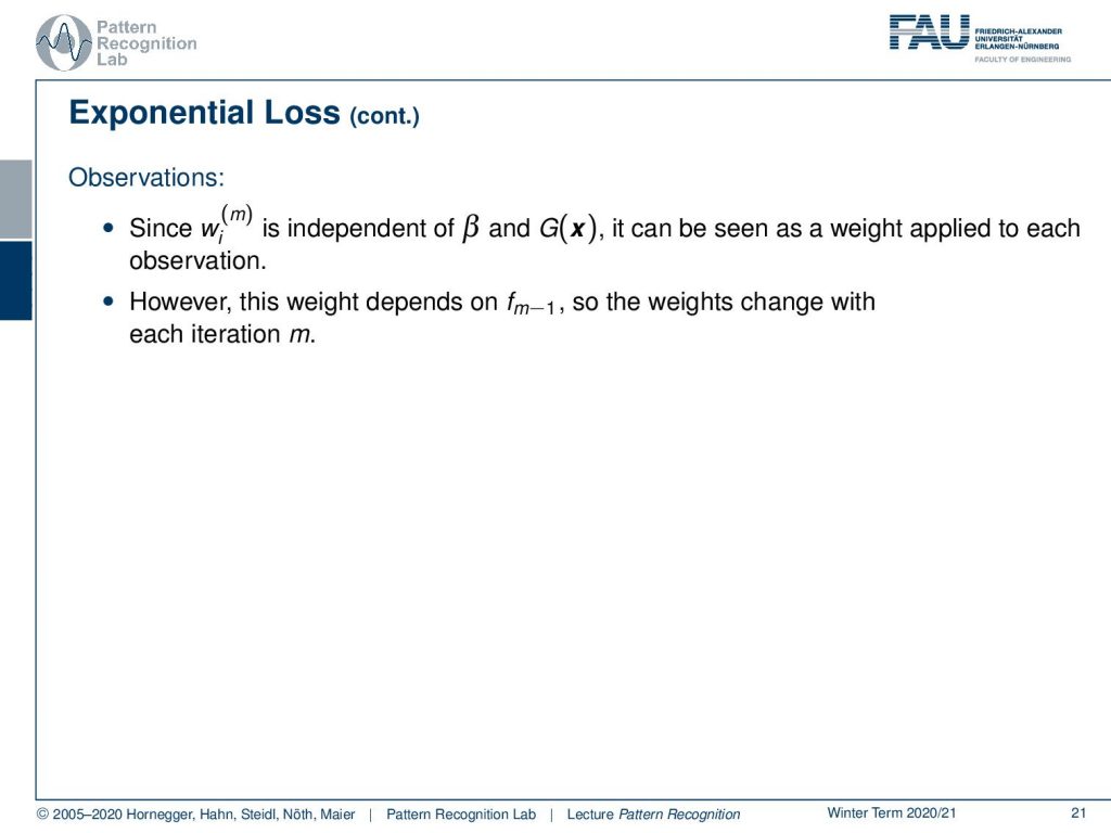
We have some observations with this. Since w_i is independent of β and G(x) it can be seen as a way that is applied to each observation. However, this weight depends on the previous functions. So the weight changes with each iteration m.

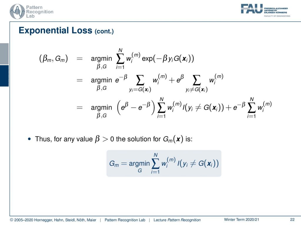
This then allows us to reformulate this problem a little. We split it up into the misclassified and the correctly classified samples. Then we can rearrange this minimisation expression. You see that we can again use our indicator function here for representing the misclassified samples. Now for every value of β greater than zero the solution for this minimization process is found as the minimization over the sum of the weight times the indicator function.

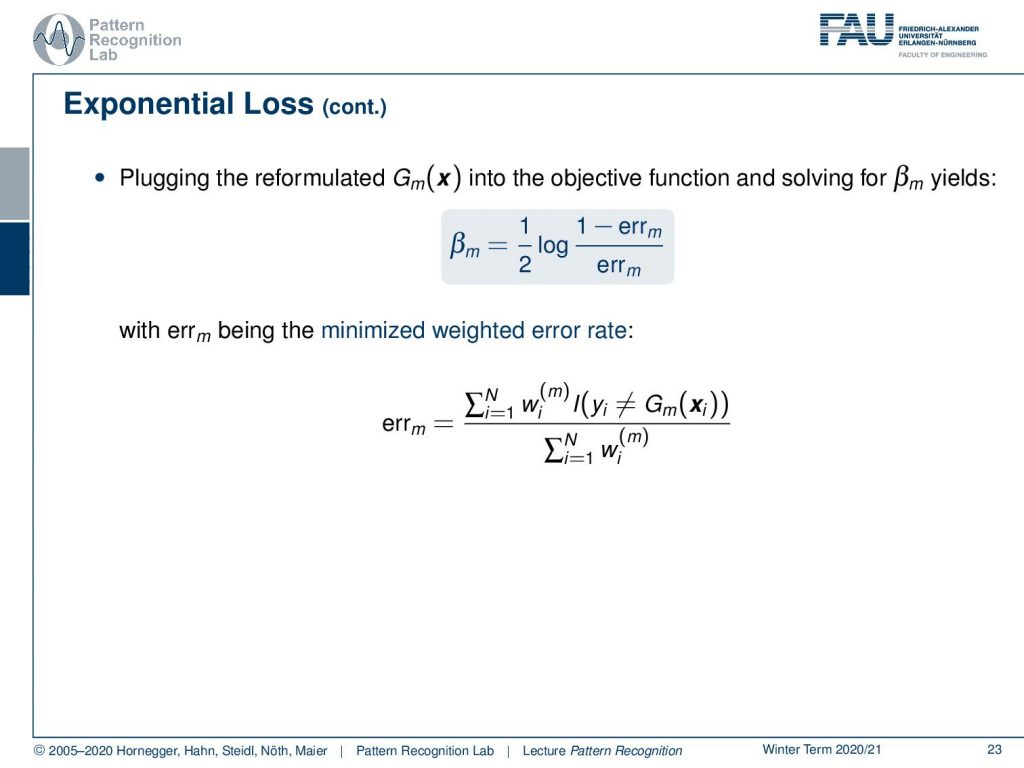
If we pluck the reformulated G_m into the objective function and solve for β_m, this yields that β_m is given as 1 over 2 times the logarithm of (1-err_m) divided over err_m. The error m is the minimised weighted error rate, and here you see that it is essentially the misclassification weight summed up, divided by the total sum over the weights.

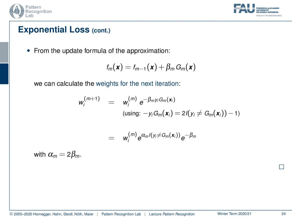
Now from the update formula of the approximation, we can calculate the weights for the next iteration. Here we can now see that we can use this identity here and derive the new weight. So here you’ll see that then α_m is going to be 2β_m. 

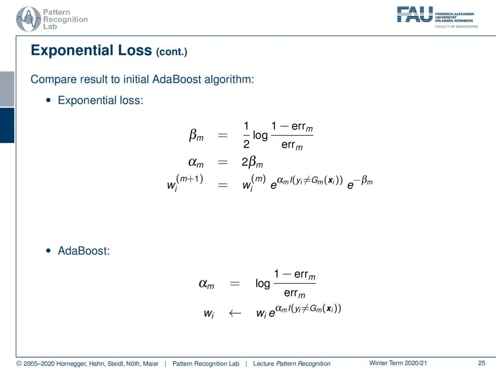
If you now compare this result to the AdaBoost algorithm, we can see that the exponential loss had these solutions for β, α_m and the weight. And if you look into AdaBoost, this had essentially an α that is very much related to the above α respectively β. Also, the weight update takes a very similar form. So you could say AdaBoost is essentially minimising the exponential loss.

Now let’s look at the losses that we want to minimise. If you have the misclassification loss that’s hard to minimise because it’s not a complex problem. But if you look into the squared error, this would be a first approximation of the misclassification loss. And then we can see that a better approximation of the misclassification loss is done here by the exponential function, the exponential loss that is produced by AdaBoost. We can also see that, if you take a support vector machine, we essentially end up with a loss that is related to the hinge loss. And we see that also the SVM is solving a convex optimisation problem to adjust a different approximation of the misclassification loss. This is quite interesting. If you’re more interested in the relation between the hinge loss and the SVM, we also have a derivation for this in our class Deep Learning. 

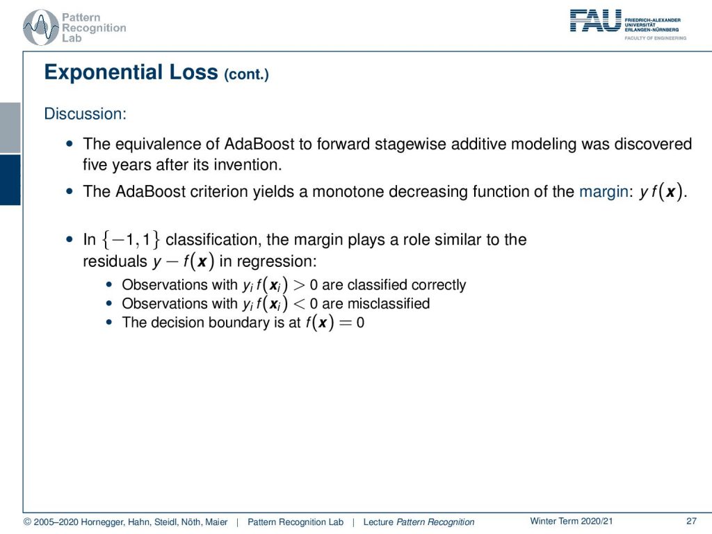
We could show that the AdaBoost algorithm is equivalent to forward stagewise additive modelling. This was only discovered 5 years after its invention. The AdaBoost Criterion yields a monotone decreasing function of the margin y times f(x). In classification, the margin plays a role similar to the residuals in regression. So, observations with y_i times f(x) greater zero are classified correctly. Observations with this term smaller than 0 are misclassified and the decision boundary is exactly at f(x) = 0.

The goal of the classification algorithm is to produce positive margins as frequently as possible. Thus, any loss criterion should penalize negative margins more heavily than the positive ones. The exponential criterion concentrates much more on the observations with large negative margins. So this is also in relation that we iteratively try to weigh up the samples that are hard to classify. Due to the exponential loss, AdaBoost performance is known to degrade rapidly in situations of noisy data and if there are wrong class labels are in the training data. So again, training data and correct labelling is a key issue, and if you have problems with the labels then AdaBoost may not be the method of choice. 

Next time in Pattern Recognition we want to look into a very popular application of AdaBoost, and this is going to be face detection. You’ll see that AdaBoost and haar wavelets together essentially solve the task of face detection very efficiently, and this then gave rise to many many different applications. And as you see in many cameras and smartphones, often the face detection algorithm that is used to detect people on the Image and show it on boxes is the AdaBoost.

I hope you like this little video and I’m looking forward to seeing you in the next one! Bye-bye. 

If you liked this post, you can find more essays here, more educational material on Machine Learning here, or have a look at our Deep Learning Lecture. I would also appreciate a follow on YouTube, Twitter, Facebook, or LinkedIn in case you want to be informed about more essays, videos, and research in the future. This article is released under the Creative Commons 4.0 Attribution License and can be reprinted and modified if referenced. If you are interested in generating transcripts from video lectures try AutoBlog.

References

1. T. Hastie, R. Tibshirani, J. Friedman: The Elements of Statistical Learning, 2nd Edition, Springer, 2009.
2. Y. Freund, R. E. Schapire: A decision-theoretic generalization of on-line learning and an application to boosting, Journal of Computer and System Sciences, 55(1):119-139, 1997.
3. P. A. Viola, M. J. Jones: Robust Real-Time Face Detection, International Journal of Computer Vision 57(2): 137-154, 2004.
4. J. Matas and J. Šochman: AdaBoost, Centre for Machine Perception, Technical University, Prague. https://cmp.felk.cvut.cz/~sochmj1/adaboost_talk.pdf

Category: Lecture Notes in Pattern Recognition