Lecture Notes in Pattern Recognition: Episode 28 – Laplacian Support Vector Machines

These are the lecture notes for FAU’s YouTube Lecture “Pattern Recognition“. This is a full transcript of the lecture video & matching slides. We hope, you enjoy this as much as the videos. Of course, this transcript was created with deep learning techniques largely automatically and only minor manual modifications were performed. Try it yourself! If you spot mistakes, please let us know!

Welcome back to Pattern Recognition! Today we want to talk a bit about the Laplacian Support Vector Machines. I think this is a pretty cool method because it allows you to implement machine learning in domains where you have labeled and unlabeled data and combine it with techniques from manifold learning and dimensionality reduction. I think it’s a bit exotic, still, it’s an exciting technique to be presented here in this video.

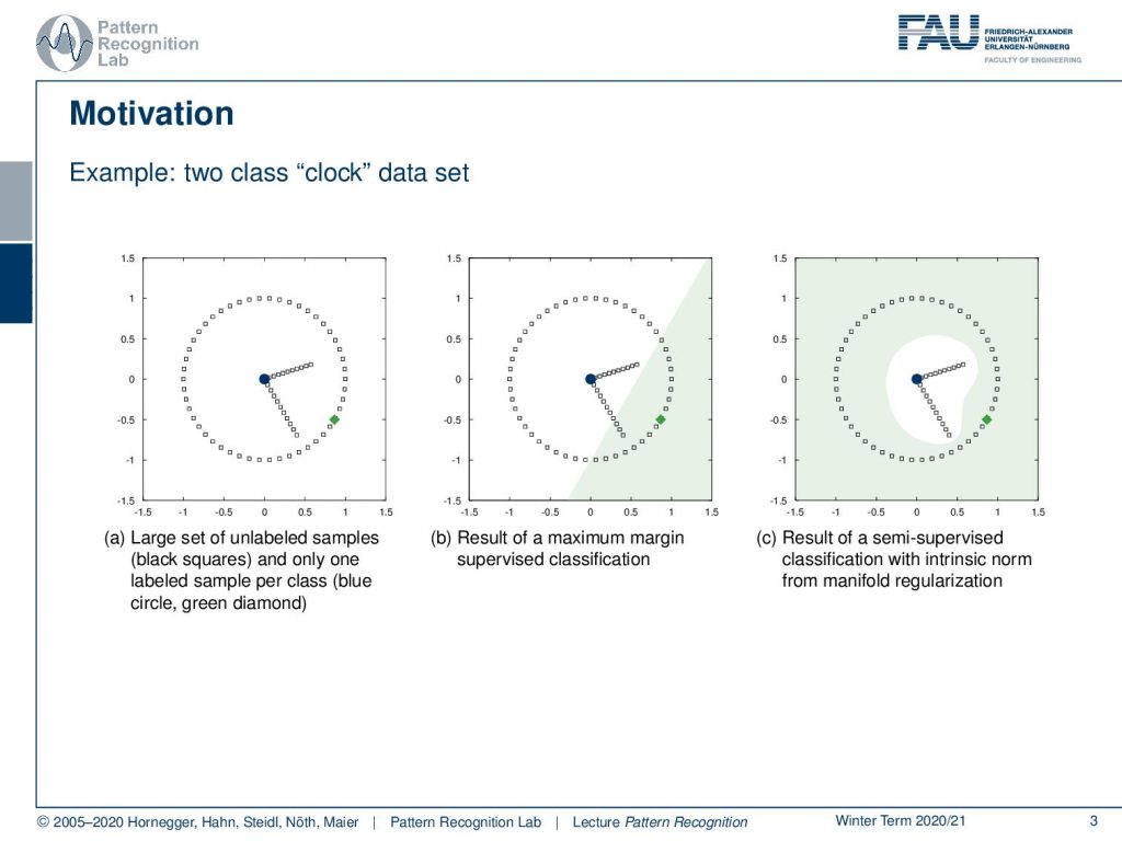
Today’s topic is the Laplacian Support Vector Machine. The idea that we want to follow here is essentially the one that you can see in this example. Let’s say you have a data set. Here this clock data set, where you only have two instances that are labeled essentially the blue and the green point. And now you want to essentially compute a decision boundary between the two. Obviously, if I take the two observations and do supervised learning with a linear decision boundary, I’ll get the decision boundary as shown in the center image. So this may be not very useful. What we want to get is exploiting the internal structure of how the points are related to each other and their geometric closeness such that we can figure out what is the inner part of the clock and what is the outer part of the clock from only the two labels. So the technique that will be able to compute decision boundaries like the one shown here on the right is the Laplacian Support Vector Machine.

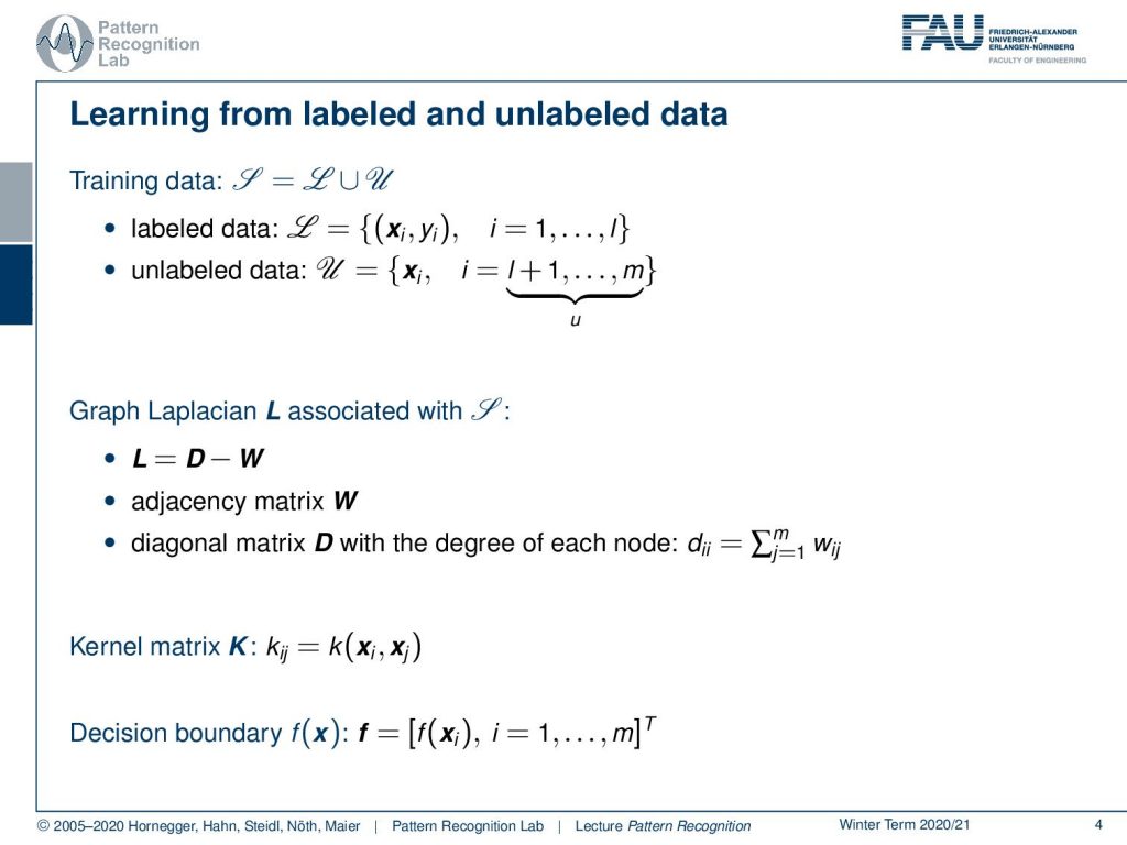
To introduce this we have to introduce a couple of concepts. First of all, our training data is now composed actually of two sets. So the complete training data is composed of ℒ, the labeled data. And you see that we have a total of l observations in the label data set. Then we have the unlabeled data, the 𝒰, that is then giving us additional observations of u up to the index m. So our entire training data set has m observations, but only l are labeled and u are unlabeled. The other concept that we need to build on is the Graph Laplacian that is associated with our entire training data set. This is given as the matrix capital L and is given as the subtraction of D–W where W is the adjacency matrix. This essentially is a matrix that tells us which elements are connected. It has some weight and tells us how strongly the two are connected. And then we essentially have the diagonal matrix D which is the degree of each node. On the diagonal, we essentially have the sum over all of the weights that are incident to that particular node. This is then called the degree matrix. And I get the graph laplacian by taking D and subtracting W. You’ll see that this matrix will become very important when we are deriving the Laplacian support vector machines. Also, we need some kernel matrix, and here we have again the notion of the kernel. So this is essentially the kernel function evaluated on some x_i and x_j. This then is all used to find a decision boundary f, and here we are essentially writing up the decision boundary f as a vector. And it’s essentially the evaluation of the decision boundary on all of the training observations. So f is then also computed for the unlabeled data, so it’s a vector of length m.

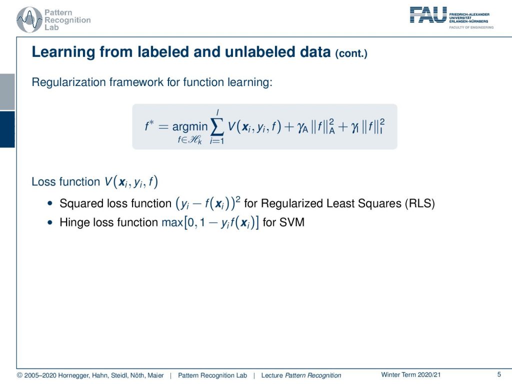
Now if we want to learn this function, we can set up a regularization framework. The function, our decision boundary, that we want to obtain is given as the minimization over a sum of a loss function. Now the loss function essentially tells us how good the fit is concerning the function of our labeled training observations. Here you can take for example the squared loss function for regularized least squares or also the hinge loss can be applied and this would then mimic essentially an SVM. 

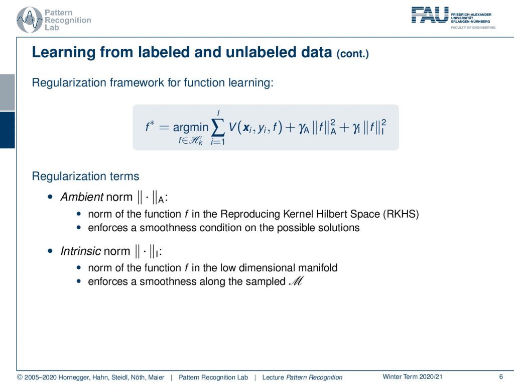
Furthermore, we have regularization terms. These regularization terms have an ambient norm. The ambient norm is essentially a norm of the function in the Reproducing Kernel Hilbert Space that we have the function defined in. The norm is supposed to enforce a smooth condition of the possible solutions. Then, we also have the intrinsic norm. Now the intrinsic norm operates on the low dimensional manifold, so the projected space where we then project our data on using the graph Laplacian. It enforces smoothness along the sampled ℳ.

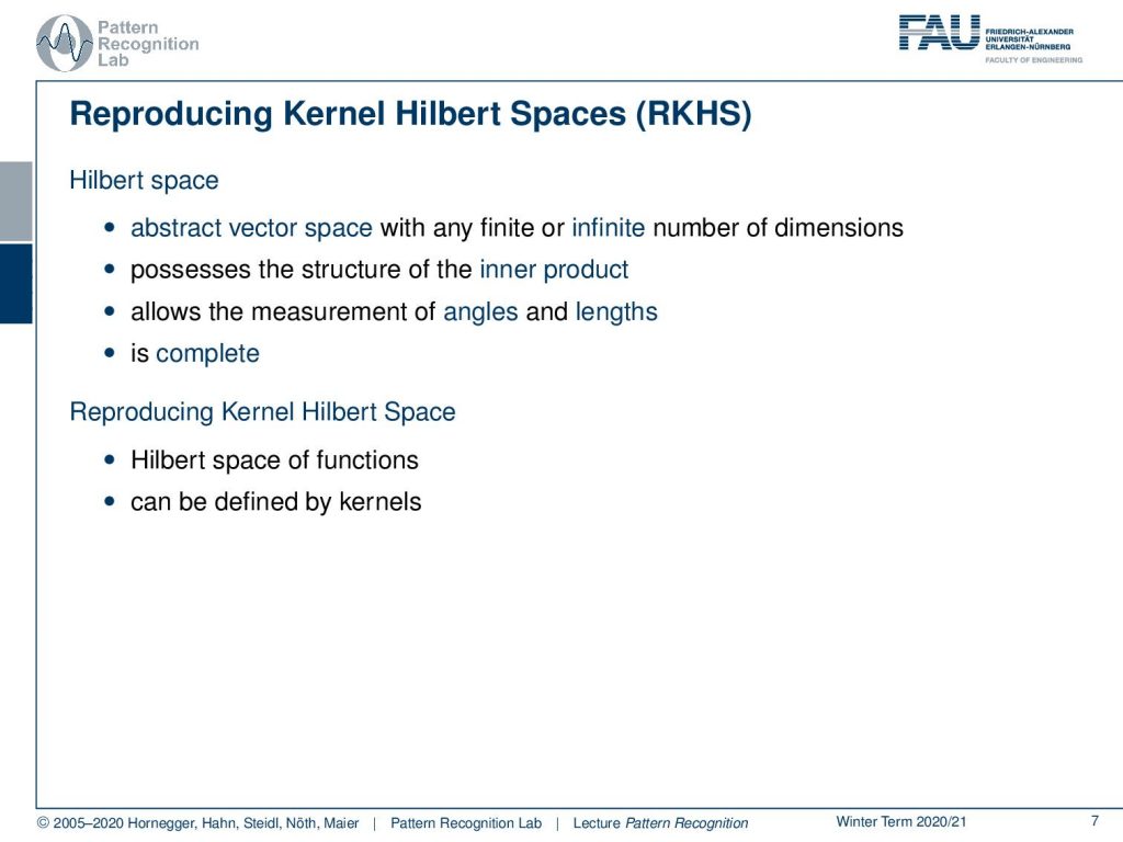
Now we already mentioned the concept of the Reproducing Kernel Hilbert Spaces. The Hilbert Space is an abstract vector space with any finite or infinite number of dimensions and it possesses the structure of the inner product. So this is very important because we want to work with kernels so it must have an inner product. And it of course then allows the measurements of angles and lengths, and it is complete. Now the Reproducing Kernel Hilbert Space is a Hilbert Space of functions and it can be defined by kernels.

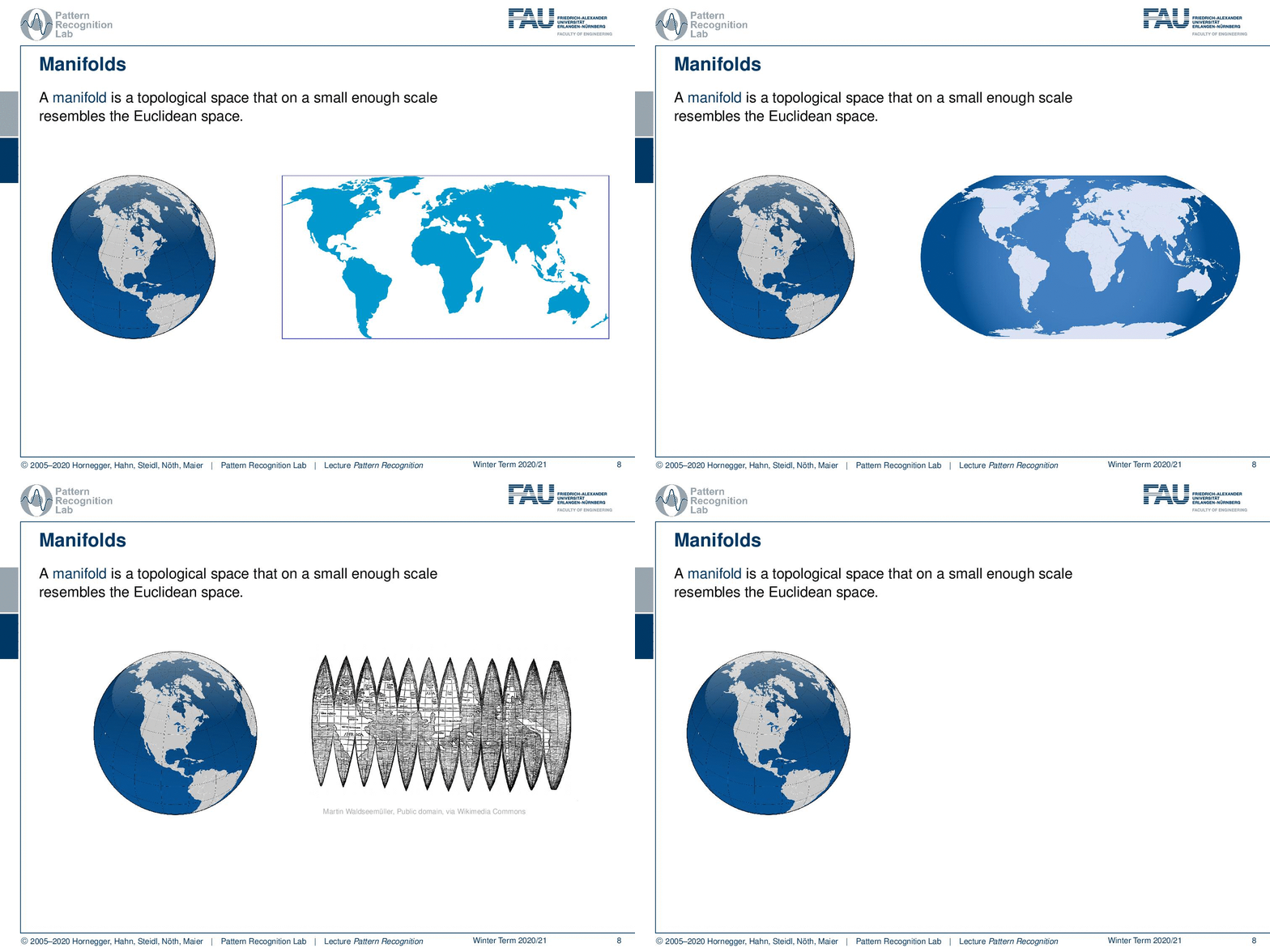
The other very important concept is the concept of a manifold. A manifold is a topological space that is on a small enough scale to resemble the properties of the euclidean space. Here, a very typical example of different manifolds is the projection of the surface of our planet. You may know this kind of projection. But then of course you can also find other kinds of projections like this one where we then enforce different properties on the manifold. And you can also essentially just unroll the surface by using this trick, like peeling the skin of a fruit. And if you do that, then you can even preserve exactly the distances. But of course, you get a non-continuous domain because you have the gaps in between where you would have to jump. But then all the distances on the surface are correctly preserved. 

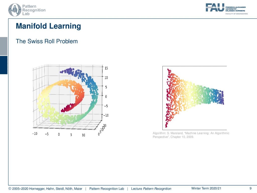
Manifold learning is essentially the idea to derive this manifold automatically. The most famous example for manifold learning is probably the swiss roll. Here you can see a set of points that are embedded in the 3D space. But their similarity is encoded in color here, and you can see that the blue points are of course more similar to each other than the red ones. What you want to do is you want to be able to map this 3D structure onto a 2D space without losing the internal information of the manifold. Solutions like this one here on the right-hand side are quite preferable. Again, things can be done with the Graph Laplacian of these point sets. And you can use the information of the Graph Laplacian to compute such dimensionality reduced spaces like the one that we show in this example.

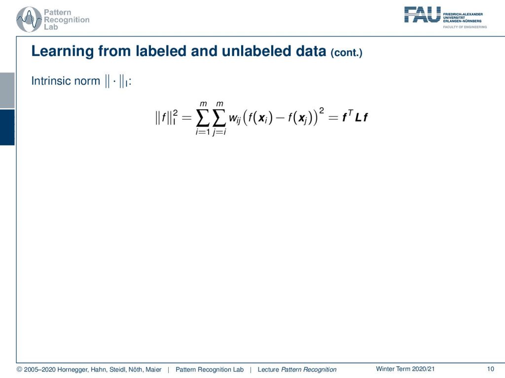
Let’s go ahead and look into learning from labeled and unlabeled data. Here we have this intrinsic norm that we know that can be applied to our decision boundary in the reduced space. And if we want to do that, we essentially have to compute the decision boundary for two observations, and then we weight them with the connection according to our graph. So we remember the w are essentially the entries of our adjacency matrix. This allows us to describe the norm with respect to the decision boundary. 

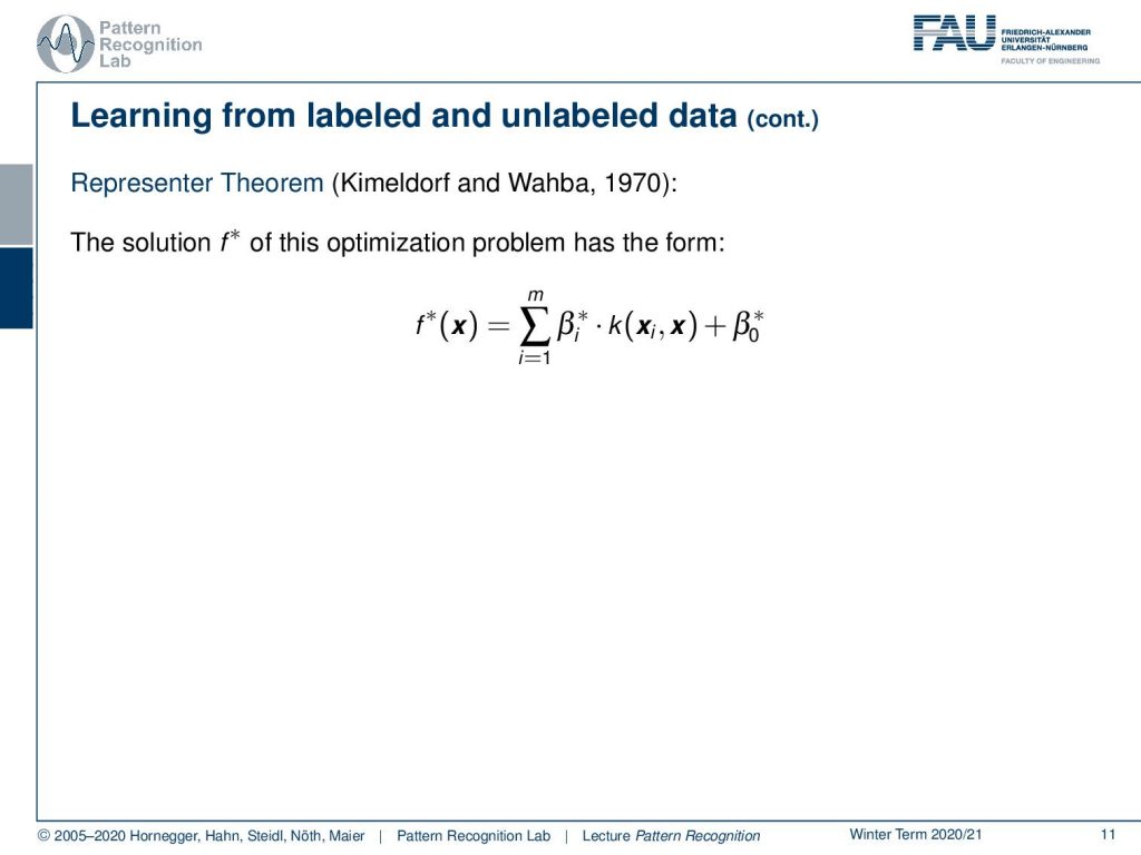
And there is the so-called Representer Theorem that tells us that the solution of this optimization problem must have the form of a linear combination of the kernels with some weights β and some β₀*. So all of the respective solutions will have this shape.

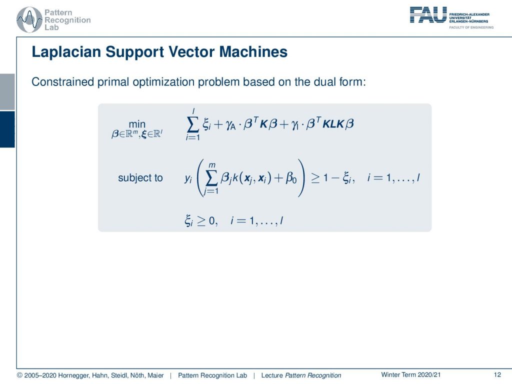
Now that we did all these observations we can rewrite our constrained optimization problem. And this brings us to the primal optimization problem here. You see now that we want to minimize our slack variables ξ, as well as our parameters β of the decision boundary concerning our kernel space and concerning our kernel space mapped onto the graph Laplacian. And of course, this then also needs to fulfill constraints, meaning that the solution of our decision boundary still maps all of the points that have a label onto the right side. And here we essentially get a formulation that is very similar to the constraints in the classical support vector machine. And of course, all of this ξ_i need to be greater or equal to zero. So this is an additional constraint.

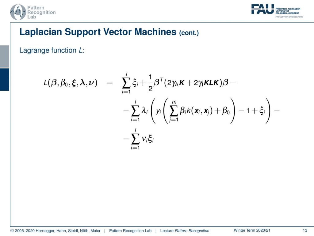
Now that we have set up the constraints we can also construct the Lagrange function. This is essentially only introducing additional Lagrange multipliers λ and ν. You see that this is essentially the same with an unconstrained kind of formulation using the Lagrange multiplier formulas. For this problem the KKT conditions hold. 

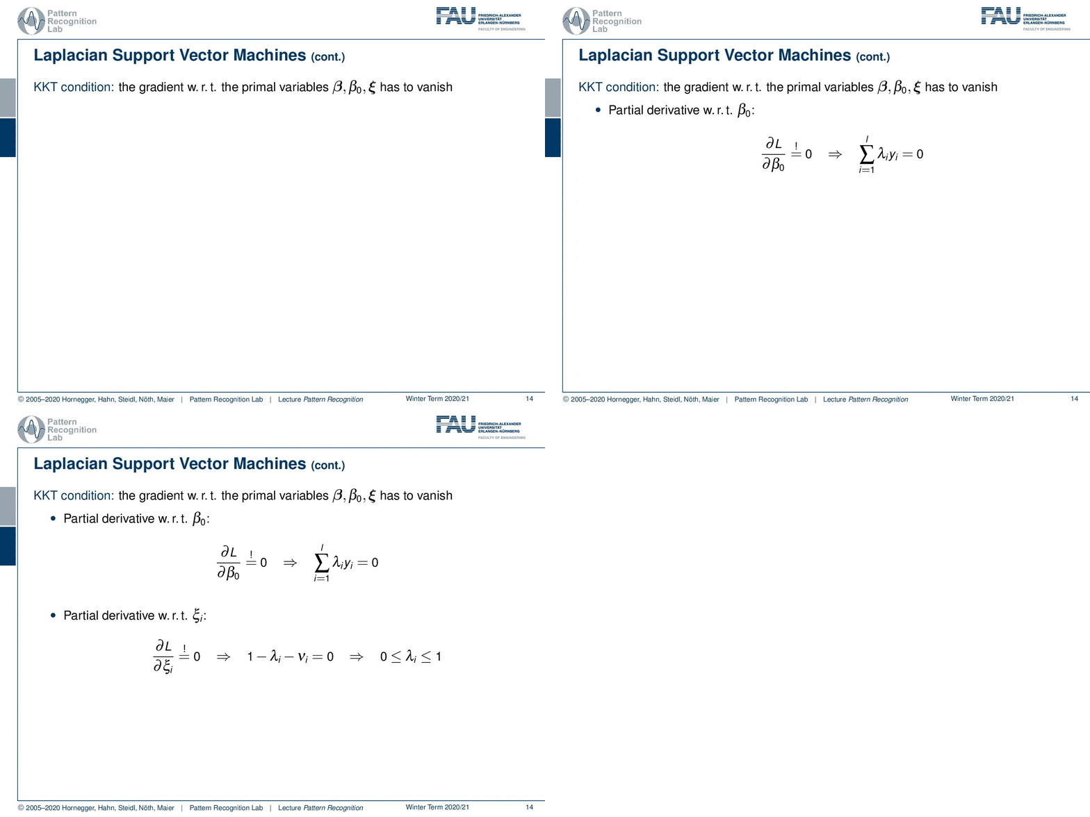
The gradient for the primal variables has to vanish. So we can compute the partial derivatives of our Lagrange function for β₀. This implies then that the sum over the labeled samples of λ_i y_i equals zero. Then we can compute the partial derivative with respect to the ξ_i’s. And this then implies that our λ’s have to be between zero and one.

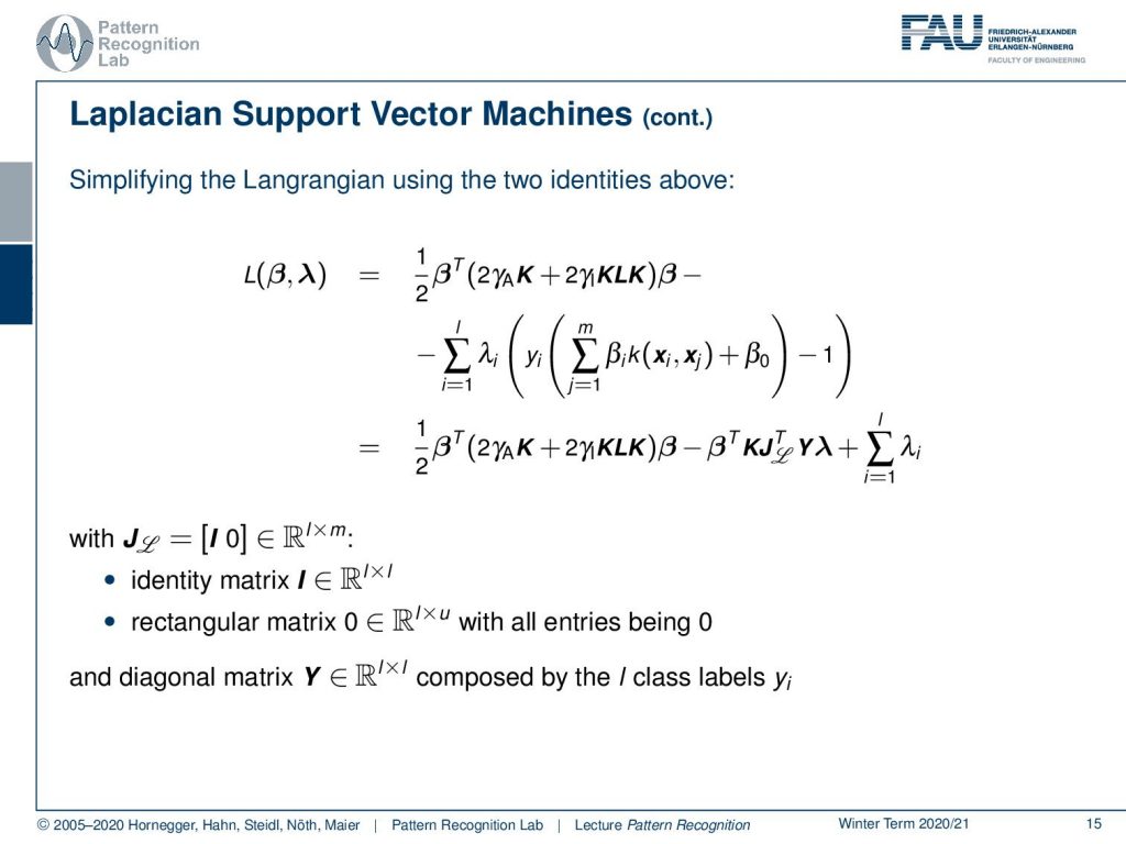
This then allows us to put in the two found identities into our Lagrange function. And we get the solution as written up here. In order to simplify this, we are introducing some matrix J. and this matrix J is the identity matrix in the space of the labeled features, and it’s a rectangular matrix of 0 in the space of the unlabeled features. This then allows us to write this up with essentially a matrix notation. And here we then also have a diagonal matrix Y that is composed of the class labels in y. This is already quite interesting. Now we can look at the Lagrangian and compute the partial derivative for our primal variable that is β.

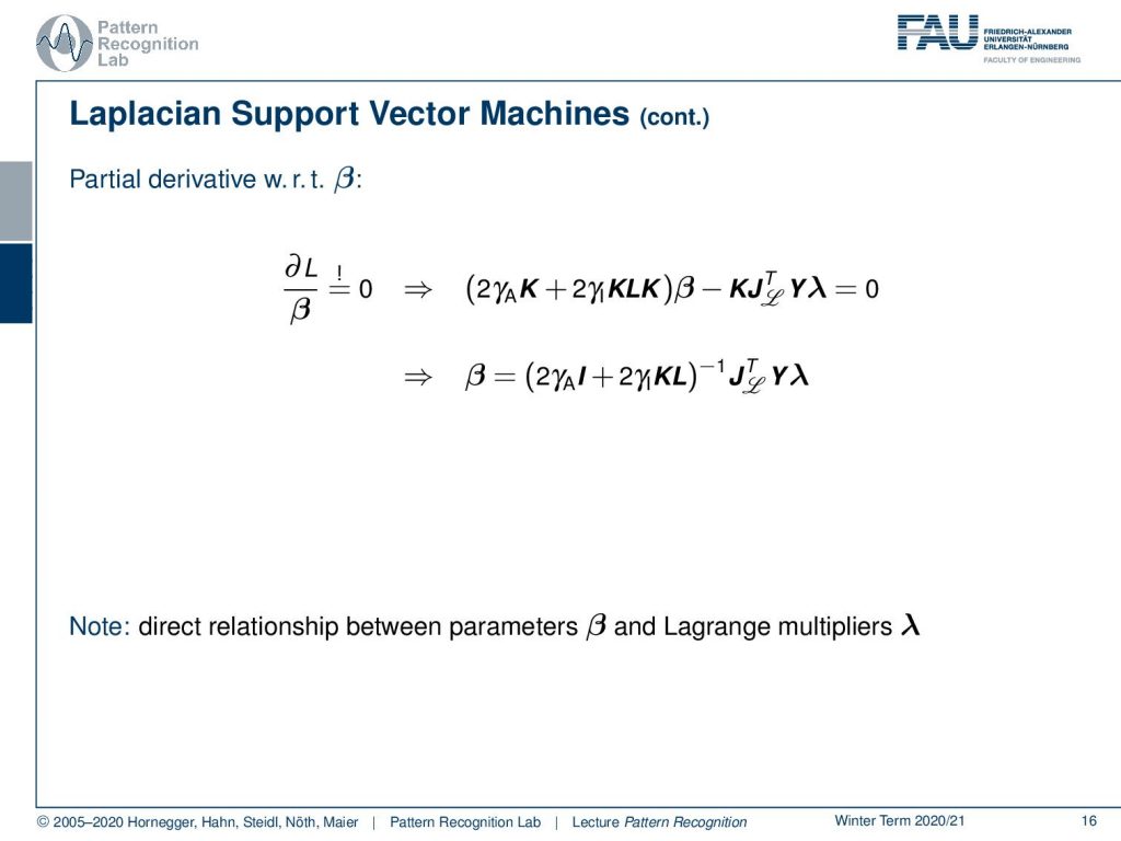
Now the partial derivative for β gives us a solution for β that is constructed as these long inverse matrix times J^T times Y times λ. This also means that our β and λ are in direct relation, which is also a very interesting observation. And of course, we can now use this identity to get rid of the β.

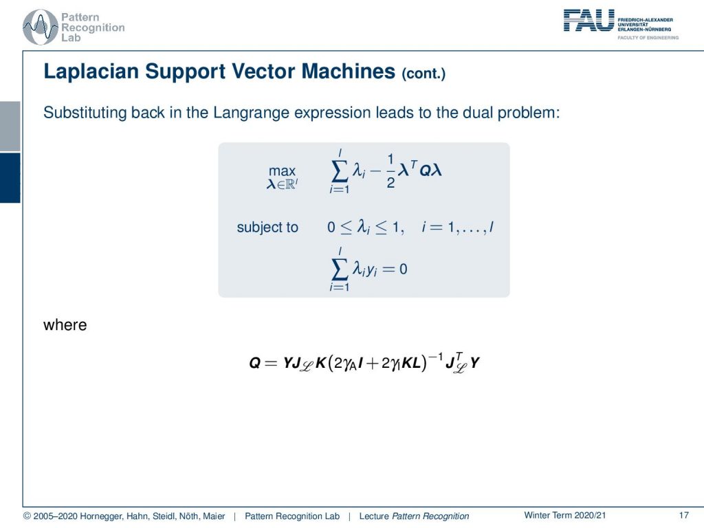
This brings us then to the Lagrange dual problem. Here we are no longer finding any β, which means that we are no longer in the domain of the primal variables but only in the duals. And here we have essentially the Lagrange variables. So we see that this can be written up in a compact form if we introduce a new matrix Q. Q is essentially this long chain of matrices that we observed earlier. And then we still have to imply our additional constraints. So there are constraints on λ_i being between 0 and 1, and that the sum over the label data set of λ_i times y_i equals 0. This is very interesting that we can essentially formulate a Laplacian SVM where we do dimensionality reduction and classification at the same time.

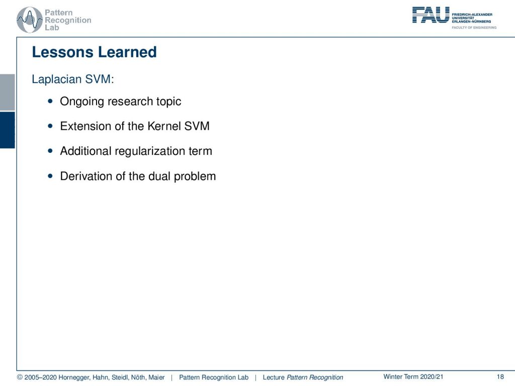
Laplacian SVM is an ongoing research topic. Right now it’s not such a hot topic anymore because a lot of what has been done is now being researched in deep learning. But you see that this formalism is also compatible with many things that we have seen in Deep Learning. So maybe that is a pretty cool research idea to look at whether we can also formulate a Laplacian SVM in the domain of deep learning frameworks. It’s an extension of the Kernel SVM and it introduces those additional regularization terms. And these regularization terms can incorporate the dimensionality reduction and the classification at the same time. We showed in this short video the derivation of the dual problem.

Next time in Pattern Recognition we want to go ahead and talk about also a very fundamental algorithm in Pattern Recognition: the expectation-maximization algorithm which is very frequently used to solve problems of pattern recognition.

I also have some further readings. Here is the original paper, the “Laplacian Support Vector Machines Trained in the Primal”. Then also “Manifold Regularization: A Geometric Framework for Learning from Labeled and Unlabeled Examples”, which are published both in the journal of machine learning research.

I hope you liked this little video, and I can tell you that the Laplacian Support Vector Machine is probably not that relevant for the exam. But still, I found it a cool method where we can then apply different ideas manifold learning dimensionality reduction and also support vector machines in the formalism using the optimization. They’re inherently compatible and this is the reason why we can combine them in this joint optimization problem. I hope you enjoyed this short video and looking forward to seeing you in the next one! Bye-bye.

If you liked this post, you can find more essays here, more educational material on Machine Learning here, or have a look at our Deep Learning Lecture. I would also appreciate a follow on YouTube, Twitter, Facebook, or LinkedIn in case you want to be informed about more essays, videos, and research in the future. This article is released under the Creative Commons 4.0 Attribution License and can be reprinted and modified if referenced. If you are interested in generating transcripts from video lectures try AutoBlog.

References

• Stefano Melacci, Mikhail Belkin: Laplacian Support Vector Machines Trained in the Primal, Journal of Machine Learning Research, 12:1149-1184, 2011

• Mikhail Belkin, Partha Niyogi, Vikas Sindhwani: Manifold Regularization: A Geometric Framework for Learning from Labeled and Unlabeled Examples, Journal of Machine Learning Research, 7:2399-2434, 2006

Kategorie: Lecture Notes in Pattern Recognition