Lecture Notes in Pattern Recognition: Episode 19 – Rosenblatt Perceptron

These are the lecture notes for FAU’s YouTube Lecture “Pattern Recognition“. This is a full transcript of the lecture video & matching slides. We hope, you enjoy this as much as the videos. Of course, this transcript was created with deep learning techniques largely automatically and only minor manual modifications were performed. Try it yourself! If you spot mistakes, please let us know!

Welcome everybody to pattern recognition!! Today we want to look a bit into the first storage of neural networks and in particular, we want to look into the Rosenblatt Perceptron. We will look into its optimization and the actual convergence proofs and convergence behavior.

So let’s start looking into the Rosenblatt Perceptron. This was already developed in 1957 and the main idea behind the perceptron is that we want to compute a linear decision boundary. We assume that the classes are linearly separable and then we are able to compute a linear separating hyperplane that minimizes the distance of misclassified feature vectors to the decision boundary. So this is the main idea that is behind Rosenblatt perceptron. 

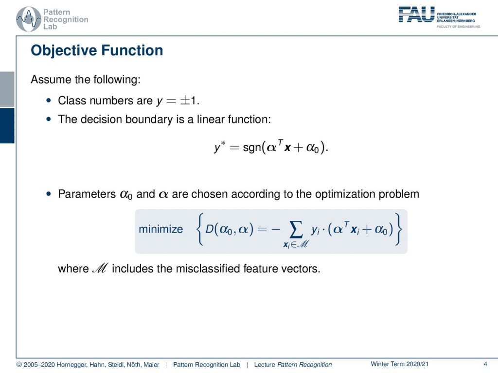
In the following, we assume that the class numbers are plus and minus one, and the decision boundary is a linear function. It’s given as y* equals to the sine of α α^Tx plus α_0. So you could say the α is the normal vector of the hyperplane and α₀ is essentially the offset that is moving the plane away from the origin. So, we essentially compute the sine distance of the vector x to this hyperplane, and then we only map to the sine of the sine distance which is then either minus one or plus one. We’re essentially only interested whether we are on the one side or the other side of the plane and this can be mapped by the sine function. Now if we want to optimize this problem and essentially determine optimal parameters for α and α₀ then we can determine by the following minimization problem. So we define some function D of α₀ and α and this is given as minus the sum over the set M where M is the set of misclassified vectors. Then we compute y_i. So this is essentially the ground truth label times α^Tx_i plus α₀. So if you look at this equation carefully you understand that y_i is the ground truth label so it’s either 1 or minus 1. And you see here then if I compute α^Tx_i plus α₀ I’m computing the signed distance. So we know that for a misclassified sample the two will have exactly the opposite sign. So you see that we essentially will get a negative value for the bracket then we will have a positive value for y_i because only in this case this would be misclassified. Of course, we can essentially flip the sign on both samples and we will also get a misclassification then. So only in the case where both have the same sign, we would have a correct classification. This means that everything every element of the sum has a negative sign and this is why we’re multiplying with -1 in front of the sum. Because only then we will get positive values so now you see that if we minimize this we’re essentially minimizing the loss that is caused by all of these misclassifications. 

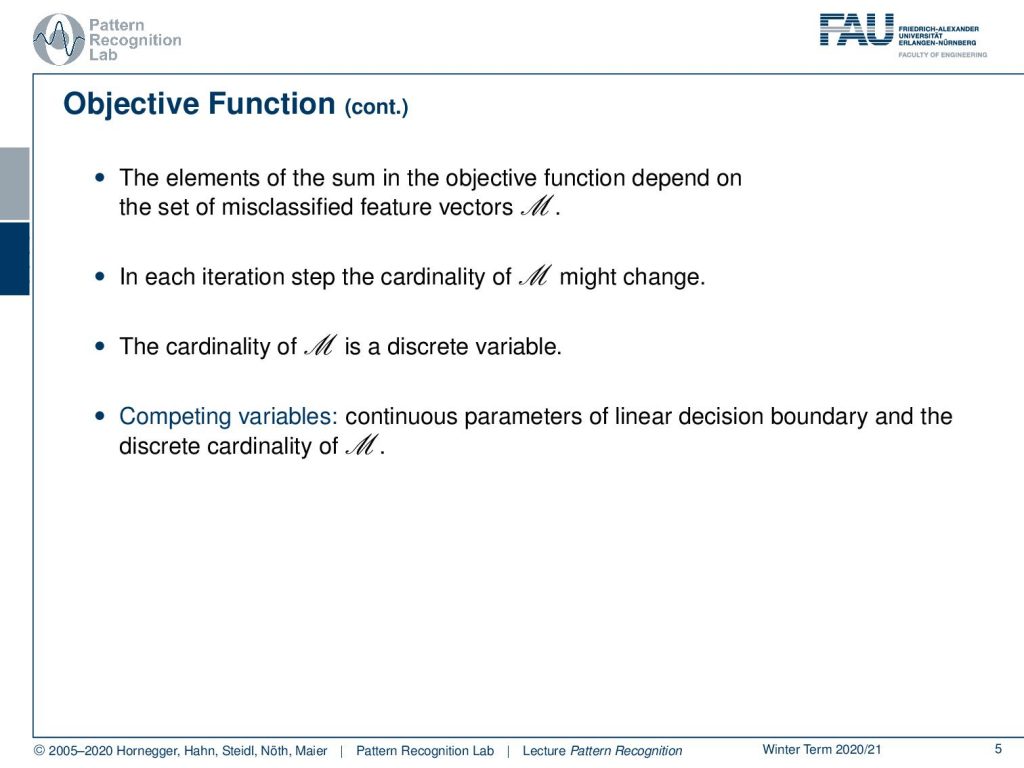
We essentially see now that the elements of the sum depending on the set of misclassified feature vectors. This essentially can change in every iteration. So every time I change the decision boundary and changing the set of misclassified samples. This is a huge problem because the set will change probably in every iteration. So the cardinality of M is a discrete variable and we kind of have competing variables we have the continuous parameters of the linear decision boundary and the discrete cardinality of M.

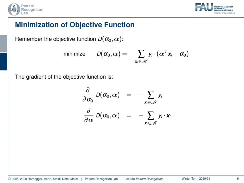
So, let’s look at this objective function that we seek to minimize. We already explained this in detail and if we now want to minimize we of course need to compute the gradient of this objective function. You see if I compute that with respect to α_0, it is simply the sum over all the y_i in the misclassified set. We have the minus sign still in front and if we compute the partial derivative with respect to α you can see this is minus the sum over y_i times x_i.

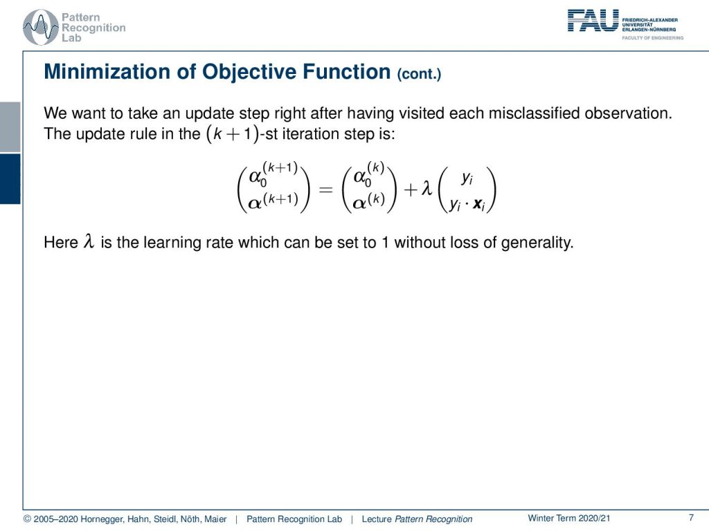
Now we can essentially look into the update rule. Let’s look into the special case where we update after each visited misclassification then we essentially get a new estimate of our α₀ and α in every observed misclassification. We immediately choose to update so we update from k to k plus 1. You see now that in brackets we write the new iteration step and we choose this vector notation. We see that this is of course the previous iteration of what we’ve seen in step number k. Then we have plus λ which is essentially the step size of our optimizer times y_i. In the other entry of this vector, we have y_i times x_i. Generally, the λ can be chosen also to 1, which is a simplification of the update step. 

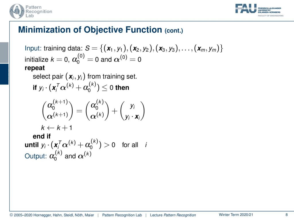
So, the procedure would then end up in having some input with training samples with the different x_i and y_i in the set S. Then we initialize for example with α0 in iteration 0 with 0 and the vector α in iteration 0 with all 0s and we initialize of course k with 0. Now we repeat and select a pair of x_i y_ifrom the training set. Then we compute the distance to the classification boundary and multiply it with the membership. And if this less than zero so in this case, we have a misclassification then we compute an update and the update is simply the old vector plus the observed pair in this vector notation. Then we get the new parameter set and we also increase the index k. Then we repeat this until we have positive values for all our samples. This means that all of our samples are classified to the right decision boundary. So you see this is a very neat way of writing up this signed distance multiplied with the class membership to produce always positive values for correctly classified samples and negative values for misclassified samples. So the output finally is α0 at iteration k and α at iteration k and of course, we require everything to be classified correctly. This means that this algorithm will only converge if the set of observations can be separated by a linear decision boundary. If this is not the case we will iterate until infinity. So the algorithm will simply not stop.

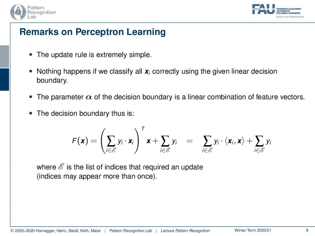
So, this update rule is of course extremely simple. If we classify everything correctly then essentially nothing will happen and the parameter α of the decision boundary is essentially a linear combination of feature vectors. This is an interesting observation. Let’s look into this in some more detail. So we see that the decision boundary can now be formulated in the following way. We observe that α can actually be replaced with the sum over all the samples y_i times x_i transpose and then x the new observation plus the sum over all the y_i. This would be essentially equivalent to the α and α0 as we’ve seen previously. Now that we know this we can also reformulate this and pull the x into the bracket and then we essentially see the decision boundary is given as a sum over the y_i times the inner product of the observations and the new sample plus the sum over all y_i. This is a very interesting observation. So we also have something that you should keep in mind here. We have some set E and the set E is essentially the list of all indices that required an update. So, we essentially store the entire training process in this list E and this also means that some indices may appear more than once. But if we consider this then we can write the entire decision boundary simply as a linear combination of all the training observations. Also, a pretty interesting concept and you will see that this concept will appear again in later lectures when we talk about support vector machines. You will see that support vector machines solve this problem much more elegantly than the Rosenblatt Perceptron. 

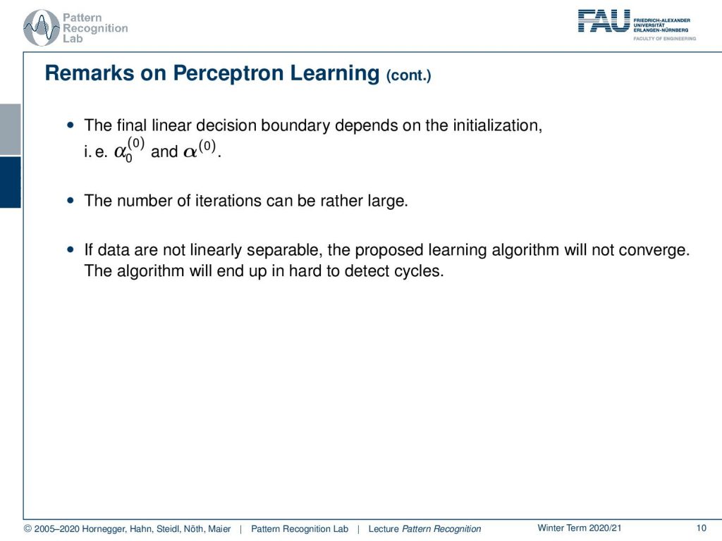
Also, the final decision boundary is linear and it depends on the initialization. So, depending on how I choose the α0 and α in the initial step I will get a different convergence result and I will get a different decision boundary. Also, the number of iterations can be rather large. So, in this very simple optimization scheme we might have many update steps and as i already mentioned if the data are not linearly separable the proposed learning algorithm will not converge. This will then essentially result in cycles and this may be hard to detect in the proposed algorithm.

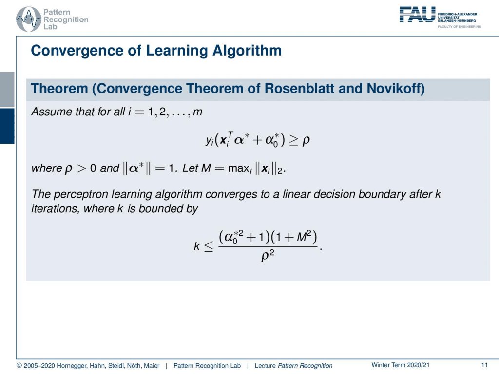
There is also a convergence proof for this algorithm and this is also introducing already interesting concepts that we will later reuse in support vector machines. The idea for this convergence theorem was also given by Rosenblatt and Novikoff. The idea that they propose is that if you have a linearly separable set of points then you can essentially use this distance to the optimal hyperplane. So, the optimal hyperplane is now described as α* and α0*. Then you can see that these variables form the decision boundary so you have the inner product with the x_i and this gives you the sign distance to the optimal separating hyperplane. This is then again multiplied with y_i. So, this will always be a positive value. This essentially gives us a signed distance on the right side of the decision boundary for all our observations and then essentially they postulate some variable ρ and ρ is now just a scalar but it is a lower bound to this distance to the hyperplane. This means essentially that there is some kind of margin, some kind of minimal distance, and this minimal distance is very important for the convergence. If I have two point sets that are far apart from each other then this ρ will be rather large and if I have two point sets that are close together then ρ will, of course, be very small. This ρ is very crucial for the convergence of the algorithm. Also, note that we choose α* to have a norm of one so this is really a normal vector and then we also introduce some variable m this is again a scalar and m is simply the longest L2 norm that appears in the training data set. So this is simply the maximum over i of all x_i and the L2 norm of that. So, if we define those quantities then we can give an upper bound for the number of iterations, and this upper bound is given for k the number of iterations. You can see that this is α₀* to the power of 2 plus 1 times 1 plus M square divided over ρ square. So you see that the value of α₀* is very important then the maximum norm that appears in the training data set is kind of important. This will increase the number of iterations but the distance between the optimal hyperplane and the samples will then decrease the number of iterations. So the larger the margin between the two sets, the more easy the algorithm will find a solution. So, this is an interesting observation also interesting is that the dimensionality of the features doesn’t appear at all in this bound. So, this bound is completely independent of the dimension of the actual feature space, also a very interesting observation.

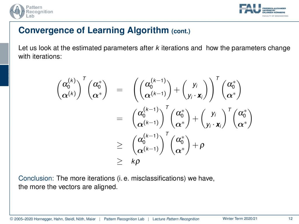
So, let’s look into this bound, how it’s being constructed and the first thing that we want to look at is essentially the inner product of the current set of parameters and the optimal ones. If we look at this inner product then we can of course see that the constellation that we found in k is created by a previous observation k minus 1. Because we’re iterating right and we did this update with the vector y_i and y_i times x_i. So, we can easily split this up this is our update rule. That’s perfectly fair to do it. Then we can move in our optimal decision boundary and now let’s look at the right-hand part of this update step. Here you see that we essentially do the projection of our point onto the hyperplane and it’s multiplied with y_i. So, here we are computing exactly the quantity that we’ve seen earlier. So, the quantity that we are projecting the point onto the hyperplane and multiply it with y_i and we’ve already seen that this has a lower bound. So this is again bounded with a lower bound by the minimum distance that is between the optimally separating hyperplane and every point. So we can plug this in here in ρ and then we also see that we have several of those update steps. So this brought us here and we see that we can essentially repeat this process all the k times that we needed to find the particular update step. And in all the k steps there is this minimum step size that we have to go which means we generally have a lower bound for this inner product with k times ρ. This also means the more iterations and more misclassifications we have, the more the vectors will be aligned. so if we do misclassifications then this will also help us with aligning the vectors to each other. What else can we do? 

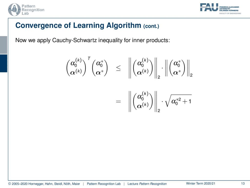
Well, let’s look at the upper bound for this inner product. So this is again the inner product of the current parameter set and the α*. So the optimal separating hyperplane and here we can now apply the Cauchy-Schwartz inequality for inner products and we see that this has an upper bound by the L2 norm of the two vectors multiplied with each other this, of course, makes sense. Then let’s look again into this in a little bit more detail. We can see that we defined the norm of the star as one this means that we can spell out the L2 norm directly which is then our first zero to the power of two plus the actual norm of α* which is one. Then we can also look at this in a little more detail.

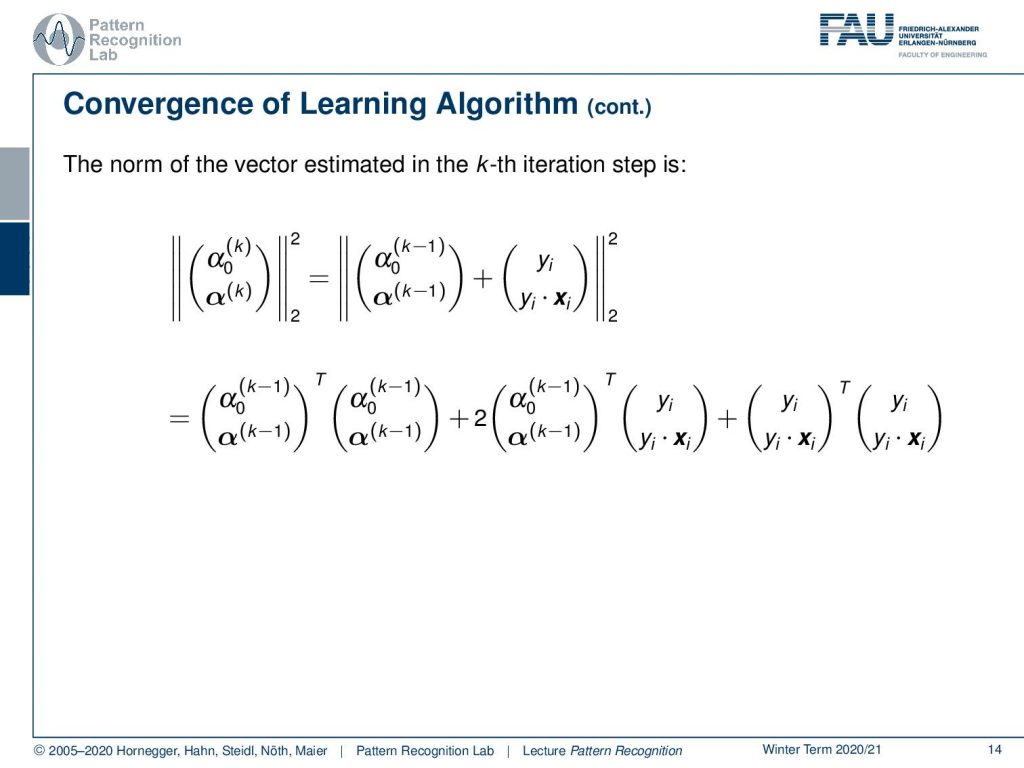
So, let’s see what we have here in the first term we have this current update step. So the L2 norm here the two norms squared now of α0 and α in iteration k and we can see again that the current configuration was of course composed of previous update steps. So, we go again into the previous iteration and see here that this is essentially constructed from the previous one plus the new observation. This is again an L2 norm. Then we can see that this L2 norm can actually be spelled out as a product of two vectors. If we do that then we see that we essentially get a quadratic term in α₀ and α. Then we get a mixed term where we essentially have α₀ α times the observation and the class label. Then we essentially have again a quadratic term that is essentially only dependent on the current observation. So, if we look closely at this then we can see that the inner part is again the projection of the sample onto the hyperplane. This is the previous set of parameters. So, we know that this term is actually negative.

So, if we look at this then you see that this inner product is again exactly this y_i times x_i transposed α^(k) plus α₀^(k). And because this was a misclassification we know that this term will always be negative. So we can essentially say if we neglect this term then we will always get an upper bound and therefore we can simply do that. We get the norm essentially of the previous constellation plus the norm of the observation that was misclassified. Now we can see that for the right-hand part we essentially have vectors x_i all the other elements are in the y_i. We can see that this inner product is then bounded by 1 plus M square because we can only have 1 and minus 1 for the y_i and of course the x_i has the maximum length of m. So, this is why we can bring up this boundary, and then we can also see that we can repeat this step of unpacking over the iterations. Of course, we can repeat this another k times which brings us then to the upper bound of k times 1 plus m square for the entire updated iteration steps. So, this is a nice upper bound for the L2 norm of the current constellation of our parameter vector. 

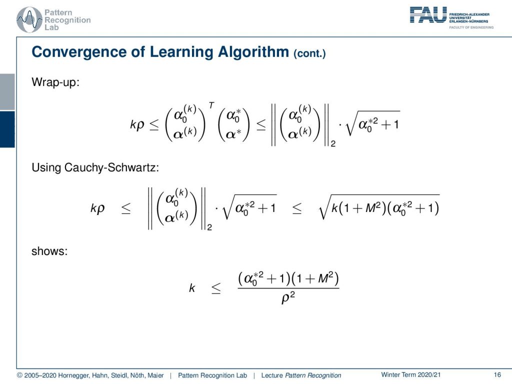
Now we can go ahead and put this back together. So, we have seen that we have this inner product of the current configuration with the optimal configuration. We’ve seen that on the left-hand side we have the k times ρ as a lower bound and on the right-hand side, we have essentially the norm of the current configuration of the parameters times the norm of the optimal configuration of the parameters. Now let’s put in what we learned earlier. So we’ve seen that we can get this upper bound of α₀^(k) and α^(k) with the k times 1 plus M square. So we can also put that back in then we essentially get the right-hand side upper bound and the left-hand side lower bound for this inner product. Now we can go ahead and rearrange the whole thing. We see now if we take this to the power of 2 and divide by k and ρ square, we get an upper bound 4k that is given as we introduced it earlier. So it’s square. So, this is already the derivation of this upper bound. 

Now, what are the implications of this? The objective function changes in each iteration step. The entire optimization problem is discrete and we have a very simple learning rule. But remember very important the number of iteration does not depend on the dimensionality of the feature vectors. This is a very important property that we have here in the perceptron and we can see that this is quite beneficial and we will use very interesting tricks when we speak about the support vector machine where we will reuse these ideas. 

So, now that we have been talking about the perceptron already, we will have a quick detour and we will talk also about the multi-layer perceptron which is essentially a combination of multiple of these perceptrons. It’s also a very popular technique right now that is also very heavily used in the techniques of deep learning. So I think we should talk about this very coarsely. If you are interested in the basic ideas we will summarize them in the next video very shortly. If you like these ideas you can probably also attend our class deep learning which will go into depth about all the neural networks and so on and all the exciting ideas there. Here in this class, we will only have a quick detour and then we will continue talking about the classical optimization strategies of machine learning and pattern recognition methods. 

Again I can recommend literature. So Pattern Recognition and Neural Networks is a very good book from Cambridge university press and again I can recommend The Elements of Statistical Learning.

I also prepared some comprehensive questions that can help you with the exam preparation. I hope you liked this little video and I’m looking forward to meeting you in the next one. Thank you very much and bye-bye!!

If you liked this post, you can find more essays here, more educational material on Machine Learning here, or have a look at our Deep Learning Lecture. I would also appreciate a follow on YouTube, Twitter, Facebook, or LinkedIn in case you want to be informed about more essays, videos, and research in the future. This article is released under the Creative Commons 4.0 Attribution License and can be reprinted and modified if referenced. If you are interested in generating transcripts from video lectures try AutoBlog

References

1. Brian D. Ripley: Pattern Recognition and Neural Networks, Cambridge University Press, Cambridge, 1996.
2. T. Hastie, R. Tibshirani, and J. Friedman: The Elements of Statistical Learning – Data Mining, Inference, and Prediction, 2nd edition, Springer, New York, 2009.

Category: Lecture Notes in Pattern Recognition