
These are the lecture notes for FAU’s YouTube Lecture “Pattern Recognition“. This is a full transcript of the lecture video & matching slides. We hope, you enjoy this as much as the videos. Of course, this transcript was created with deep learning techniques largely automatically and only minor manual modifications were performed. Try it yourself! If you spot mistakes, please let us know!
Welcome back to Pattern Recognition! Today we want to talk a bit about regression and different variants of regularising preparation.
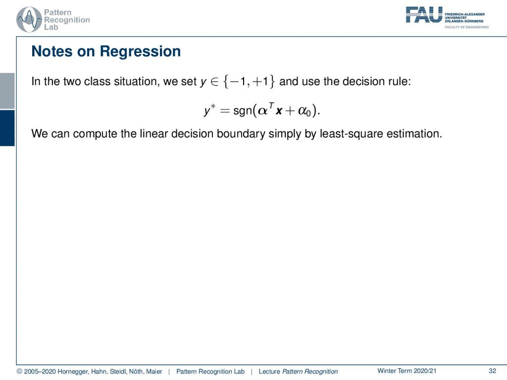
You see here that this is the introduction to regression analysis. The idea here is that we want to essentially construct a linear decision boundary. In our two-class set, this would then be sufficient to differentiate whether we are on the one side or the other side of the decision boundary. Therefore, we compute the sign distance αT x + α0 to that particular hyperplane. Then the sign function just tells us whether we are on the one side or the other side of this decision boundary, as we’ve seen and the previous Adidas example. Now the idea is that we can compute this decision boundary simply by least-square estimation.
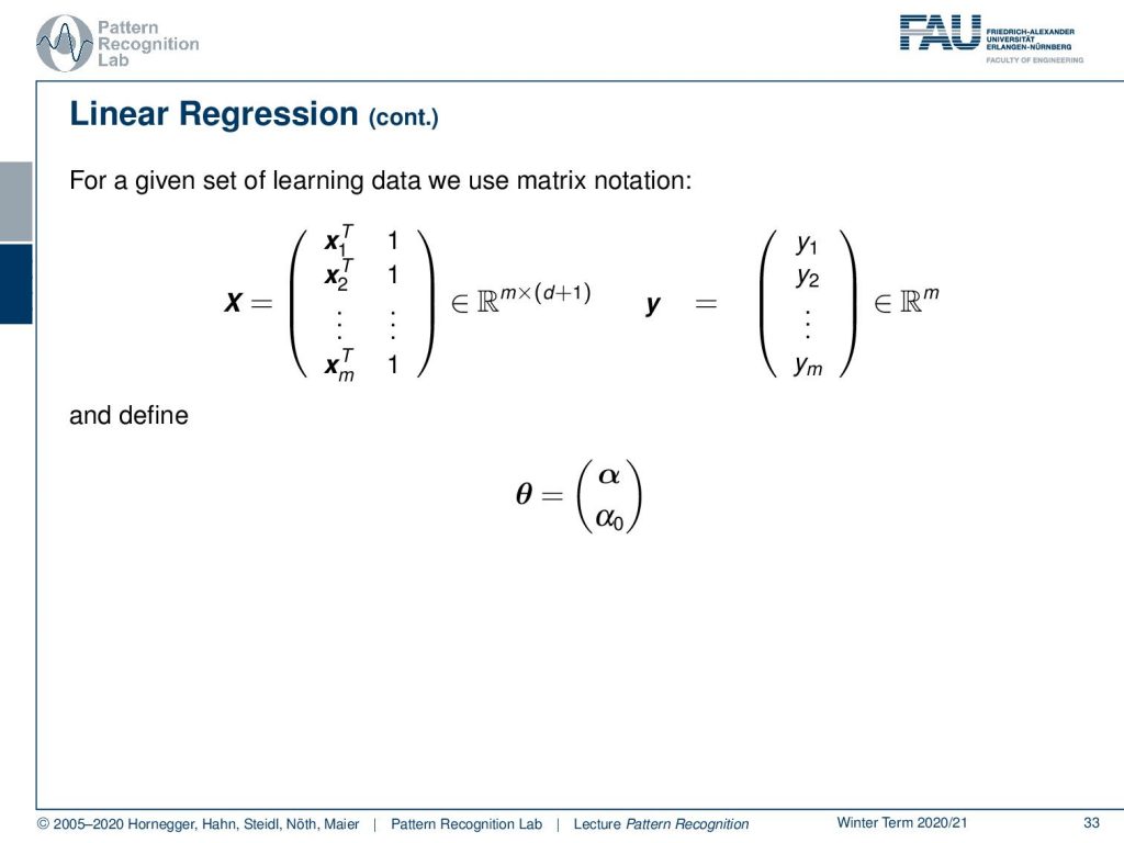
The idea here that we want to follow is that we essentially convert our entire training set into a matrix and a vector. Here, the matrix is given by the individual feature vectors transposed, and we add a column of one at the very end. This gives us the matrix X, and this is then a matrix in an m x (d + 1) dimensional space. So, d is the dimensionality of our feature vector, and m is the number of training observations. This is then related to some Vector y. In this vector y, we essentially have the class memberships of the respective feature vector. Now we want to relate those two with a parameter vector θ, and θ now is composed of the normal vector α and our bias α0.
Now, how can we do the estimation? Well, we can simply estimate θ to solve the linear regression problem. So we essentially take the matrix X multiplied with θ and then subtract from y, take the L2-norm to the power of two, and compute the minimum over this norm with respect to θ. And you can see, then we can break up this norm and built the least-square estimator. So we can write also this square either as a sum of the individual components, or we can break up the L2 -norm squared with this product of the two terms and transpose. So this is essentially an inner product, and it doesn’t matter which solution you take. If you do not take the partial derivative with respect to θ and do the math, then you will find the solution of the so-called pseudoinverse. So, this is the very typical Moore-Penrose pseudoinverse that is given as XTX, and this inverted times XT times y. This will essentially be a solution that will give us an inverse, which will enable us to compute the parameter vector θ from our observations X and y. One thing that you have to keep in mind here is that this will work if the column vectors of X are mutually independent. If you have a dependency in the column vectors, you will not have full rank, and then you will run into problems. One way how to solve this then is to take the singular value decomposition. And another way is, of course, that you apply regularization. We’ll talk about the ideas of regularization in the next couple of slides.
The questions that we want to ask is: why should we prefer the Euclidean norm, the L2 norm? Will different norms then lead to different results? Which norm and decision boundary is the best one? And, can we somehow incorporate prior knowledge in this linear regression?
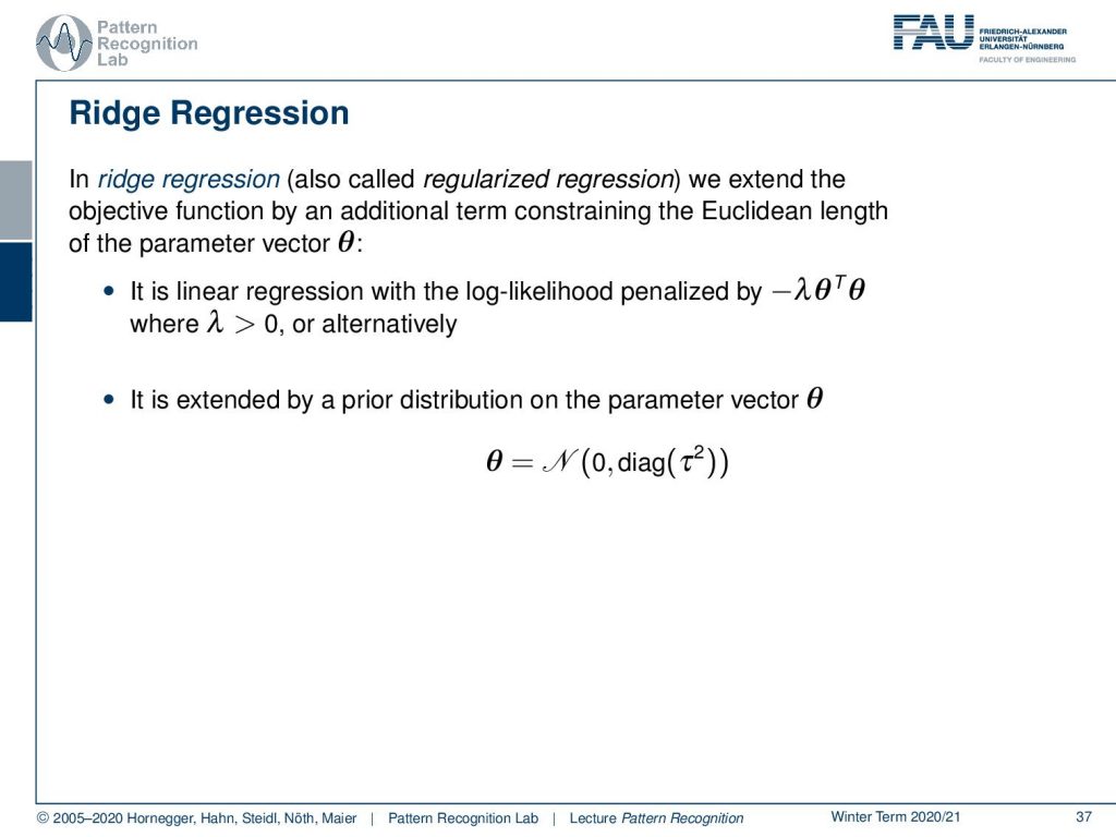
This then leads to the concept of ridge regression, or regularized regression, where we extend the objective function with an additional term. For example, you can constrain using the Euclidean length of our parameter vector θ. So you could then say that you have a linear regression with the log-likelihood. This is penalized by -λ θT θ, so the L2 norm of θ, and you set λ to be greater than 0. We will see an equivalent formulation. You could say we extend our estimation with a prior distribution on the parameter vector θ. And we assume θ to be distributed in a Gaussian way, where we essentially have a zero mean and a diagonal covariance matrix with some factor τ2 as the variance. Let’s look into the details of how we can see that this is true.
We start with the regularized regression. We use the Lagrangian formulation here, so you see that our constraint, that our norm should be small. It’s simply added with the Lagrangian multiplier in here. And then we can see that we can further rearrange this, so we can again express the norms as in a product using this transport notation. This then allows us to compute the partial derivative for θ. And again, I can recommend doing the math on your own. You can have a look at the Matrix Cookbook. This is also a very good exercise to practice with because you will see that you find the following solution. You set the partial derivative for θ to 0, and then you solve for θ. And this essentially gives you θ̂, and θ̂ can be computed as XT X plus λ, the unity matrix, and the whole term inverted times XT y. If you compare this to the classical pseudoinverse, you see that we essentially have only the λ times the unity matrix.
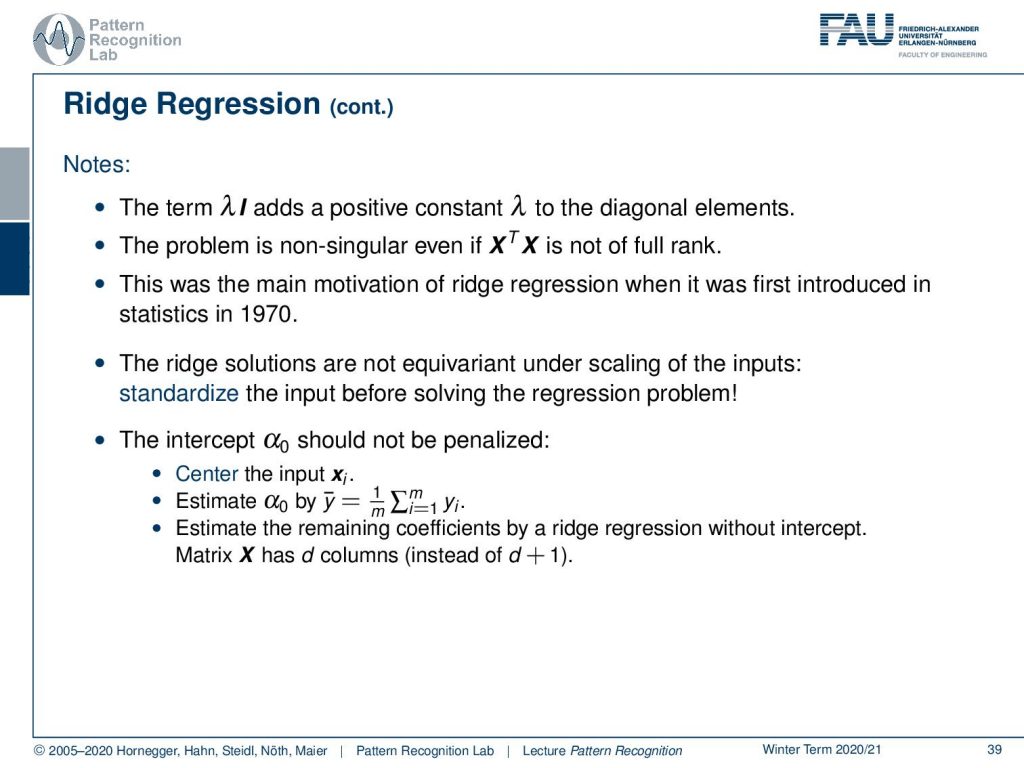
This essentially means that you’re adding a small positive constant on the diagonal elements. So this is all that your ridge regression is introducing in this case. But this is a very nice result, because then the problem is non-singular, even if XT X is not full rank. Because when you add the small constant to the diagonal, this will cause your problem to suddenly have full rank. This is a very interesting approach to do this, and this actually was the main motivation of ridge regression when it was first introduced in statistics in 1970. This way you can stabilize your solution, and you will always find a full rank matrix here. This is a very nice way to regularise your solution. And we’ll see that you can apply these regularization ideas not just for regression but in many many different optimization problems. This is a very classical way of getting difficult, unstable problems into some constraint domain, where you actually can get the solutions also pro biasedly. The ridge regression solutions are not equivariant under the scaling of the inputs. So you should standardize the input before solving the regression problem. One approach could be that you essentially not penalize the intercept of α0. This can be done by centering first the input using the mean of xi, and then you estimate first your α0 by some estimate of the average of your classes. And this is essentially an average of the prior. So you compute the mean over class memberships, and then you can go ahead and estimate the remaining provisions by ridge regression without intercept. This means we solve the problem, again, by using this matrix X. But you already set α as a constant, and then you solve it on a d-dimensional problem. So you have now d columns, instead of d+1. So we’re not adding this column of one in the variant.
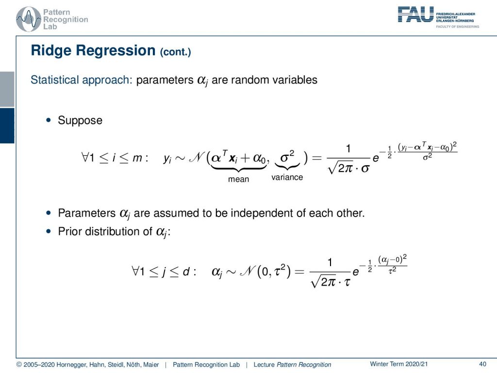
This is also in relation to statistics. And actually, we can also consider our parameters αj as random variables. Now, let’s suppose that our actual observations, the yi, are normally distributed, and the actual decision boundary is the mean. So you have the αTxi + α0. This is then modeled by some variants σ2. The parameters αj are assumed to be independent of each other. So we model this essentially using a unit covariance matrix. Then this leads to a prior distribution of the αj with a zero mean, and then essentially for every j, a standard deviation of τ2. Let’s assume these things. This then allows us to go ahead and write this up as a normal distribution for both of the cases. One is mean free, the other one has essentially the decision boundary set as a mean.
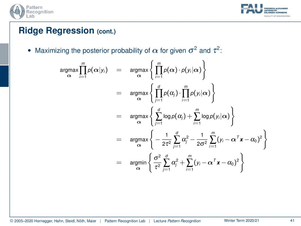
Then we can go ahead and use a maximum posterior probability. We can see now that we want to maximize the probability of α, given the observations yi. Now we can of course apply the base theorem. There we rewrite this then as the probability of observing α at all times, the probability of observing y given α. This then can be rewritten. We can split up the product here, and see that the prior on the α is only dependent on the dimension, whereas the probability on the yi is dependent on the number of observations. So we can split the two terms and write them up as a multiplication. Then we can go ahead and apply or trick with the log-likelihood. The log-likelihood then yields us essentially a maximization of the logarithm of the priors on the left-hand side, and then the logarithm of the P(y| α) of the constrained probabilities on the right-hand side. Now let’s use our Gaussian assumptions here. You’ll see that this will essentially cancel out the logarithm. We remove all of the terms that are independent of α because they are irrelevant for this maximization. Then we see that we simply have on the left-hand side the square of αj summed up and scaled with the variance of the parameters here. On the right-hand side, it’s essentially the sum over the distances to the decision boundary. This is then also summed up over all of the observations and scaled with the respective variants in this distribution. And we see this is a maximization, so we can multiply this also with a constant. Let’s multiply this term by -2 times σ2. This will convert this entire thing into a minimization. And you can also see that the two will cancel out, and we just have one factor that is σ2 over τ2 at the first term on the left-hand side.
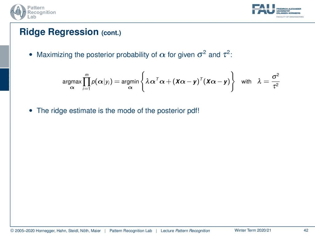
Now, if you look very closely, you can see that we can bring this again into the matrix notation that we used earlier. So we can see that this is essentially the inner product of the α vectors. That is the first term. We can then replace the σ2 and τ2 as λ, so we certainly bring in our variable λ again. The right-hand term is again an L2 -norm. So you essentially see that the ridge estimate that we talked about earlier with the L2 norms is essentially the mode of the posterior probability density function if we assume that they are distributed with Gaussian normal distributions. So this is linked. This is already a pretty cool observation. If you’re preparing for the exam, this is something that you should be aware of.
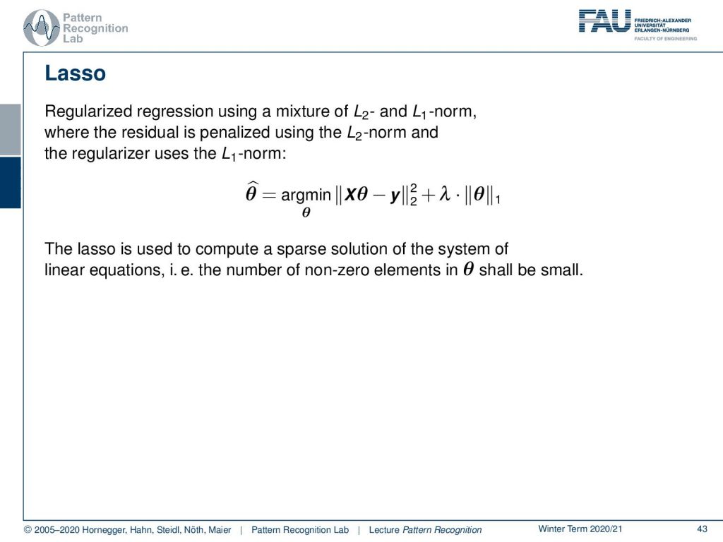
Let’s go ahead and look into other forms of regularization. We’ve seen that the ridge regression is using an L2 norm, but obviously, we can also use other norms for the regularization of our parameters. The so-called Lasso is a very typical choice, which is then applied to the parameter θ. The idea of Lasso is that you’re trying to get sparser solutions for the parameter vectors. This is very often used to compute sparse solutions of the system of linear equations. So, you try to achieve a large number of zero elements in the solution vector. You want to have only very few non-zero elements.
So, what did we learn? We learned about principal component analysis. We used linear discriminant analysis with and without dimensionality reduction. Both, PCA and LDA, are computed using eigenvector problems, you just have different matrices on which you apply them and a different form of normalization on the process. And of course, for the LDA you will always need the class membership. Otherwise, you won’t be able to compute any kinds of inter and intra-class covariance matrices. We brought in two alternative formulations. We have the rank reduced one and the Fisher transform, which is the classical approach of formulating the problem. Also, we looked into linear and ridge regression methods for classification.
This then already brings us to the next lecture. In the next video, we want to talk about different kinds of norms. You’ve already seen that if you look into the Lasso, we suddenly had this L1-norm popping up. I think at this point it is highly relevant that we discuss the properties of different norms and which effect they have actually on the optimization. You see, we now formalized a lot of the basics, the actual optimization problems. And in the next couple of videos and lectures, we will look into how to optimize these problems very efficiently. Therefore, also regularisation is a very big deal. In order to understand regularisation, you have to understand the norms that we are regulating with.
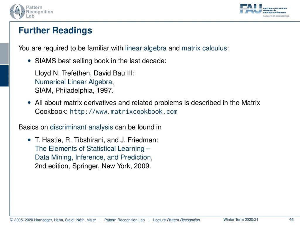
I do have some further readings again. The best selling book in the last decade from science is “Numerical Linear Algebra”, the Matrix Cookbook you’ve seen. We are using this on various occasions, it’s really useful to find very good matrix identities. And then also the basics of discriminant analysis in “The Elements of Statistical Learning”.
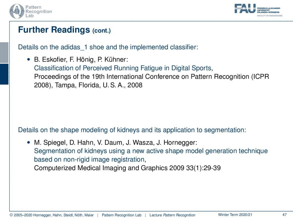
If you got interested in our applications, you see here the work by Björn Eskofier about the classification of perceived running fatigue and digital sports. This has been presented on ICPR, the international conference on Pattern Recognition in Tampa Florida. Also, one nice thing about science is that, if you can travel, conferences typically take place at very nice locations. Tampa Florida is definitely worth going to and having a conference there. The other topic that we talked about in applications was shape modeling. This you can see in the picture of Martin Spiegel. There, they are essentially presenting this kidney modeling approach with active shape model generation techniques. This was presented in Computerized Medical Imaging and Graphics in 2009.
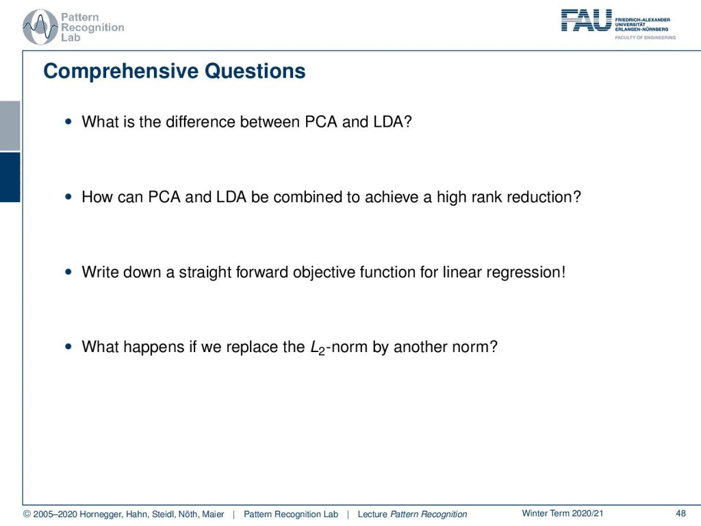
I also have some comprehensive questions, and I hope they can help you with the preparation for the exam. Thank you very much for listening!
If you liked this post, you can find more essays here, more educational material on Machine Learning here, or have a look at our Deep Learning Lecture. I would also appreciate a follow on YouTube, Twitter, Facebook, or LinkedIn in case you want to be informed about more essays, videos, and research in the future. This article is released under the Creative Commons 4.0 Attribution License and can be reprinted and modified if referenced. If you are interested in generating transcripts from video lectures try AutoBlog.
References
Lloyd N. Trefethen, David Bau III: Numerical Linear Algebra, SIAM, Philadelphia, 1997.
T. Hastie, R. Tibshirani, and J. Friedman: The Elements of Statistical Learning – Data Mining, Inference, and Prediction. 2nd edition, Springer, New York, 2009.
B. Eskofier, F. Hönig, P. Kühner: Classification of Perceived Running Fatigue in Digital Sports, Proceedings of the 19th International Conference on Pattern Recognition (ICPR 2008), Tampa, Florida, U. S. A., 2008
M. Spiegel, D. Hahn, V. Daum, J. Wasza, J. Hornegger: Segmentation of kidneys using a new active shape model generation technique based on non-rigid image registration, Computerized Medical Imaging and Graphics 2009 33(1):29-39