System Theory – Introduction to Signals and Systems

These are the lecture notes for FAU’s YouTube Lecture “Medical Engineering“. This is a full transcript of the lecture video & matching slides. We hope, you enjoy this as much as the videos. Of course, this transcript was created with deep learning techniques largely automatically and only minor manual modifications were performed. Try it yourself! If you spot mistakes, please let us know!

Welcome, everybody to a new episode of Medical Engineering and today we want to continue talking about our lecture, and in particular, we want to start introducing systems theory. So I know there will be a bit of Math but I try to put in a lot of examples such that you can follow this more easily. So this will be a couple of lecture videos where we actually do have math in there. But I will try to make it as easily digestible as possible. So looking forward to exploring with you some systems theory.

So our topic today is system theory and we want to start with a short recap. Why we actually need systems theory and what kind of images we’re dealing with? What kind of data we’re dealing with in medical imaging and why system theory might be useful to understand the general basics of our systems? 

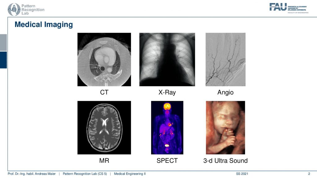
So you remember that we had different imaging modalities and those modalities had very different appearances. They had very different contrasts and we’ve seen the examples from CT to x-ray to Angiography, MR, SPECT, and also Ultrasound. So we’ve seen we have many many different modalities and all of those modalities have very different properties.

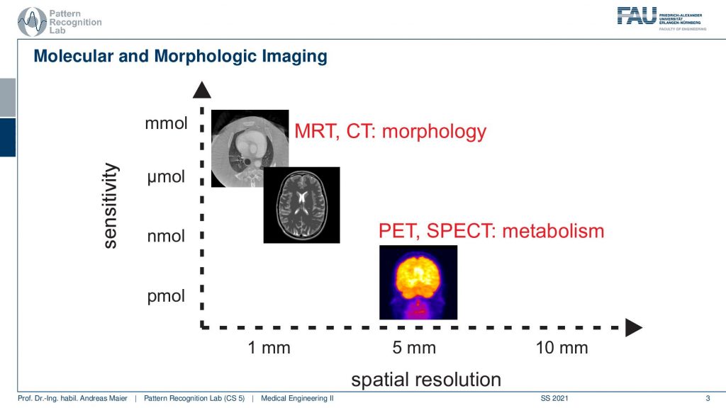
In particular, they’re very different in terms of sensitivity. So the number of molecules or the amount of different material you can visualize in terms of contrast. We’ve seen that MRI and CT need kind of lots of material in order to generate contrast but they also have a very fine resolution. On the other hand, nuclear imaging like PET and SPECT can visualize very small quantities of tracer for example but they come at a course resolution. So you see that all these kind of things they come with certain trade-offs and systems theory is essentially a theory that allows us to understand those trade-offs. 

So this is generally a theory that allows us to work with different things that are processing let’s say information or signals. 

Now if we want to understand that we have to talk about signals and systems first. So signals and systems are the key components of systems theory. 

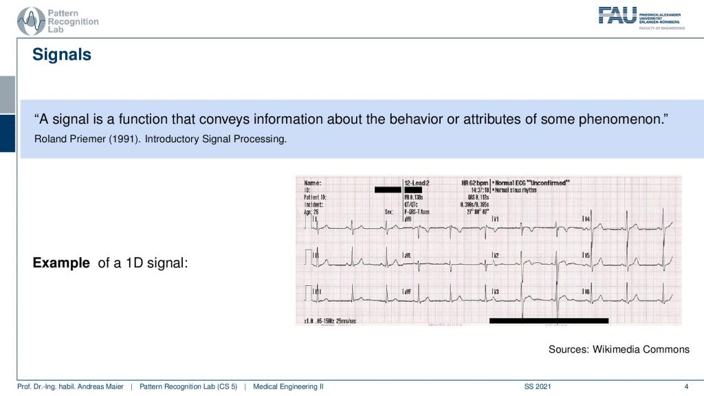
Now, what is a signal? A signal is a function that conveys information about the behavior or attributes of some phenomenon. This sounds a rather coarse and complex definition as an example I brought to you here an ECG. So ECG is a signal and this is essentially a voltage that is measured from the body and we use it to measure how the heart behaves inside of your body. So this is information. The information that we want to have is we want to diagnose the heart and therefore we look at the voltage that is generated by small electrons that are attached to your body and they deliver this kind of signal.

Now with the system, we want to somehow process that information and in an abstract sense, a system is something that processes the signal. 

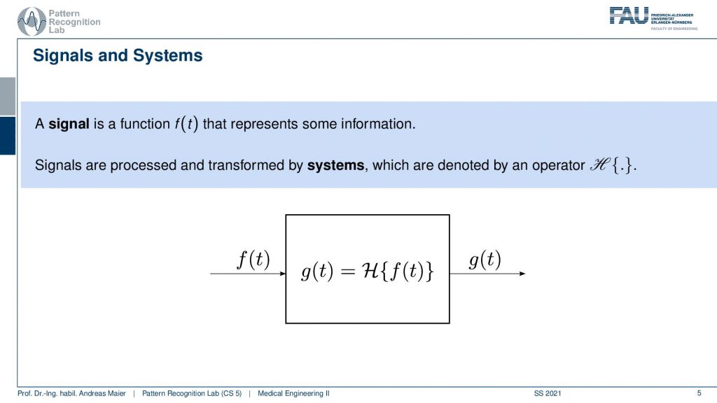
So the signal is generally a function that represents some information and the signals are processed and transformed by systems. This is generally denoted at least here in our lecture slides with an operator H. So you have some function f(t). This could be the ECG that we just looked at and then you have some system and the system processes the function i.e. the signal and then generates a new signal. So this is g so we have f(t) as input. We process it with our system and the system produces a new signal. So this is the fundamental setting that we are operating in and you see that this is kind of a really big problem domain. So our system could be anything ranging from a simple sensor from the electrodes but the system could go as far as the hard that is generating then the electricity that is sampled by our sensor. The sensor is connected to a device that is then displaying the signal on the screen. So that could also be a system. So a system can be a really complex conglomerate of different processing units. Also if you think about modern AI techniques, Deep Learning and so on they essentially also form information processing systems. Everything that you’re learning here about signals and systems will also apply to very complex systems. Now in order to be able to describe these systems better, we also assign a couple of properties. 

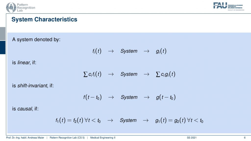
So these are characteristics of systems that allow us to find classes of comparable systems and of course we describe this with some kind of mathematics. So we can have a system and this is denoted by our operator H. It takes in some functions f_i. Now we have multiple functions that go in and we produce multiple functions that go out. So it’s not just necessarily a single function that we’re talking about. But it could also be two or, three or, more functions that are processed with this system. So it’s not just a single signal, but you can also have many many signals that are processed by the system. Now a couple of important properties are we listing here. In particular, linearity is an important one. Linearity essentially tells us that if a weighted sum of input signals is processed by the system, it’s again a weighted sum of output signals. So that’s linearity. We’ll see linearity is a very important property and it will help us if we are able to determine whether a system is linear because then we can also work with certain mathematics that allows us to describe the system more easily. Also, a very important characteristic is if a system is shift-invariant. Now this means that if you have a shift in variance system, you can shift with some variable t₀ and we subtract it t₀ in order to shift the input signal and if it is shift-invariant then this is nothing else than shifting also the output signal. So shift-invariance means that a system processes independent of the shifting of the signal. So if I shift the signal process and get the output it is identical to processing and then shifting. So this is shift-invariance. We’ll see that linearity and shift-invariance are very important properties that allow us to describe systems very elegantly if the two properties are fulfilled. We will see that in one of the next videos. Another important property is causality and here causality is a very easy concept. The causality here in this context just means that you don’t have to look into the future. So if you have some input signal then the system can process the input signal and it will be able to determine the output without having to access future information. So in this case the systems are causal. So we don’t have to look into the future so we will simply be able to process the output and generate the output without having dependencies on observations that we didn’t do so far. So you can imagine that this is a very important factor if you think about latency and dependency of systems on future observations. If you would have to look ahead then this can cause a significant delay in the output of the processing system. If you have image processing then generally causality is not such a big issue because you typically have access to the whole image domain and then it’s only a 2d shift and we can do that in an arbitrary direction. So their causality is not such a big deal. It would be if you have moving images like videos, then causality is again a huge issue. So you don’t want to be dependent on future time points.

This was kind of abstract. So let’s look at some examples.

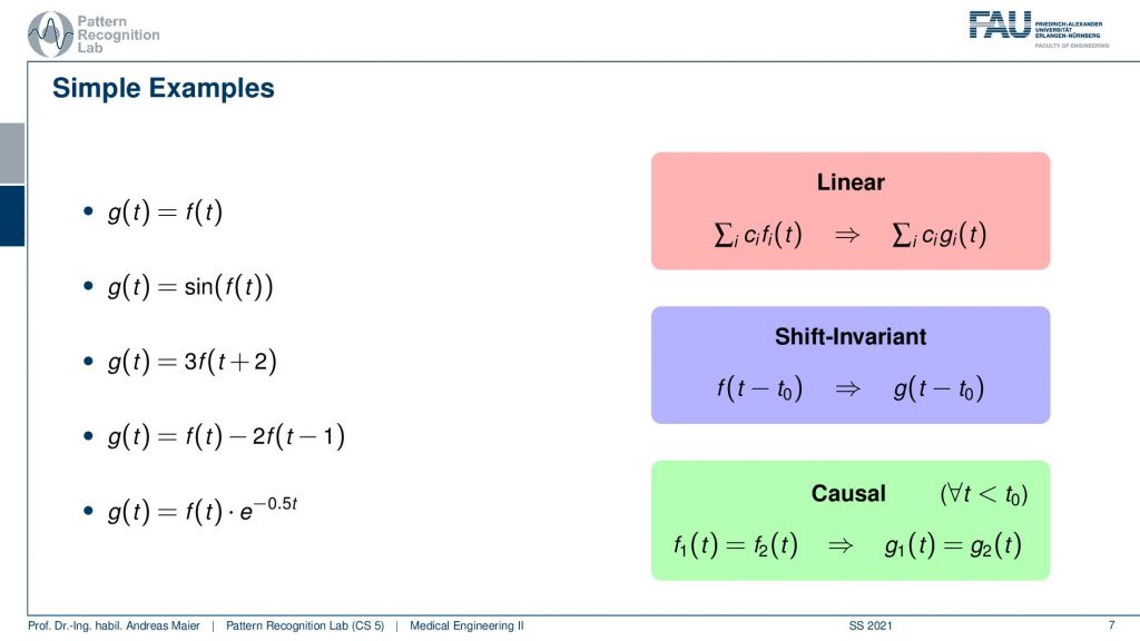
I have here a couple of examples. The first one is very easy so the output of the system g(t) is simply the input of the system. Then a second one is that we have the sine of the input function. The third one is that we shift by two and then multiply by three. So that’s also a rather easy system. The fourth system is that we essentially duplicate the function. So we have the original function minus two times the function shifted by one and the last one is we are multiplying with an exponential function that is dependent on t. So let’s look at those examples and see if we can apply here our different properties and see whether they apply.

So the identity is a very simple case and we can see if we have the identity essentially the linearity already falls out of this. So we could just plug this in and prove linearity no big deal this applies. Shift invariance again also applies. So if I shift before and after it wouldn’t do anything because we are just using identity here. So this is a linear and shift-invariant system and of course, it’s also causal because we don’t have to look into the future. Let’s still look at an example and the example that I have here it’s not the ECG because I’m using a function plotter here and you know the ECG I would have to plot from data and therefore it’s easier to take a different function. Here I’m using a sinc. So this is nothing else than sin(x) over x. You see that this is then essentially a sine that is also amplified here by the way with a factor of three. But this function here we can see that it alternates up and down and it also dampens because we’re dividing by the magnitude of x towards the outside. So we kind of can very easily see whether it’s shifted or not. So that’s very nice about this function and this is why I’m taking it as an example as input for the other systems that we’ll see in the following. So of course our identity does nothing. If I shift you can actually see that I’m plotting two functions here I’m plotting a dashed version and a gray version of the same function and you see both of them of course overlap because we have an identity. Obviously, if I shift this a bit to the front and back you see both of them still overlap of course because of the shift invariants. So no big deal all of the properties apply and we can see this in this nice visualization here.

Let’s make this a little bit more complicated and go to the second example. So here in the second example, we have the sine of the input function and this is a bit different. So if you think about the linearity the sine function has a maximum value of plus one and a minimum function value of minus one. So whatever I’m doing to this kind of function I will be clamping to minus one or to one. So this is not a linear function because if I have a superposition before applying the sine the result will be different than applying the same superposition or weighted sum after the sine. So this is going to be different hence linearity does not apply. How about shift-invariance? If I shift the sine well the function is shifted. So shift-invariance actually holds. So our function will be shift-invariant. Also, causality I don’t have to access the future here. So causality will hold too. Let’s look again into the example and I brought again our sinc function. Now you can see that we have two different outputs. So the output our g(t) is dashed while we have in gray the input function. You can see here that exactly this clamping effect is taking place. So the values that are above one get essentially transformed and they are mapped into a different space. So that we essentially get rid of the central lobe here by applying the additional sine. Now how about the shift invariants. let’s shift the input and if you see I’m shifting the input I can shift it a bit around and it doesn’t change anything because it’s shift-invariant. So we don’t have a problem here and it’s also causal because we don’t have to access the future. 

Well, let’s go to the third example. Now the third example is just multiplying with three and then you have a shift of plus two. So this is actually linear because we just have additions and multiplications, not a big thing. So our superposition or weighted sum would not be changed. That’s good. Then this is also shift-invariant because I can shift before and after it doesn’t change anything. But it’s not causal. I add 2 in the index which essentially means that I have to shift the function into the future. So this is a non-causal example and you will see that here on the next slide. You see that lobe of our central lobe of the sinc is moved to the left. So if you compute the output of the system you have to access the future. So this is a non-causal system again it shift-invariant. So if i shift the input also the output will be shifted. So that’s not a big deal. So here we have an example for something that is non-causal linear and shift-invariant.

Let’s look into the next example. so the next example is again we subtract two functions from each other. So it’s actually the same function we shift we multiply by two no big non-linearities in here. So this is actually a linear system. You also see that it is shift-invariant because we don’t have any functions in there that cause any problem with shifting. You will also see that it’s causal because we don’t have to look into the future. It’s a slightly more complex system. If you look now at the plot you can see our input is again the sinc and our system now shifts by one and then subtracts two times the function value which causes the strong negative peak on the right-hand side here. Still, it is shift-invariant. So if I shift the input the output will be shifted as well. So that’s not a big deal and we found again a system that looks slightly complex. So we can express in terms of shift-invariant linear and causal systems quite a few complex systems. But we are still able to assign these properties. So this means that we are holding all of the three properties that we have learned so far. 

Now let’s go to the last example and here we have this exponential function that is multiplied. If you remember how the exponential function looks like you see here with the negative exponent. This is essentially a decay. So everything on the right half-space of our coordinate system here will be dampened. On the other hand, everything on the left-hand side will be amplified and the t is not dependent on the actual shift. So this is neither linear because we have the exponential function and the exponential function is dependent on t but not on the shift of the function. So it will also be shift-variant. So it’s also not shift-invariant but it’s causal. So this is the only thing that applies to this system here. So let’s have a look here and as I already said you see the dampening on the right-hand side of the half-space. You see the magnification of the amplification on the left-hand side. So although our sinc is essentially just leveling out you see how the exponential function is boosting this up. So this is really an amplification that is happening on the left half-space. Now the key problem here is that the amplification is fixed to the coordinate system and not the function. So if you look now at the shifting you see that our lobe gets amplified more and more the further we go away from the zero position. This is very interesting and here you see a system that is definitely not shift-invariant. So it processes the data very differently depending on how you shifted it. So you see how shift-invariance is also a very important property if you want to describe systems.

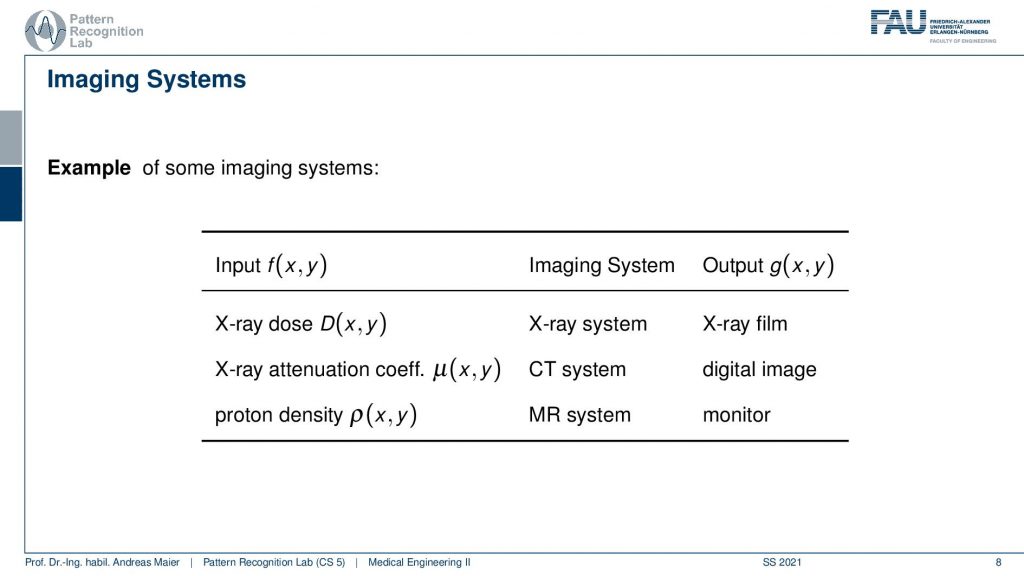
Now let’s summarize a little bit what we’ve seen here so far. We’ve seen that we have different systems- they can be anything from analog processing to digital. So it could be an x-ray dose entering your detector then the x-ray system and an x-ray film. So all of this is analog. It’s still a system and system theory applies. It could also be attenuation coefficients and then you have a computer tomography system that is computing digitally the entire image and then you have a digital image. It’s also a system – system theory applies. It could also be something like proton density, an MR system with all the rf coils and so on which is a really complex system, and still, it would be modeled by our system theory. So you see why system theory is very important for our field and to be honest you will need this throughout your entire career systems theory will apply. So this is truly fundamental to anything that you want to do in medical imaging processing systems. So please take care the next couple of videos will be very important and you will hear this over and over again in your studies. There will be several people trying to explain this to you and I hope this rather superficial way is a good start before you dig into all of the math in order to follow the systems theory. By the way, also the complex AI systems and so on also obey systems theory. So it’s not like that you can trash that if you use deep learning or artificial intelligence and so on. All the systems that are built on such techniques also have to obey systems theory.

Well, I hope you liked this short video and an introduction to systems theory, signals and system. It’s very short it’s quite superficial. You’ve seen a little bit of the math. We introduced three very important concepts that are linearity, shift-invariance, and causality, and these three things will be important throughout the entire class. So please memorize them you will see that now in the next couple of videos when we talk about essentially 1d systems for the next three videos then we’ll go to 2d and you will see still systems reapplies. Now in the next video, we want to talk about another very important concept and this is going to be the Fourier series and Fourier transforms. So there we want to think about a possible basis for function spaces and you will see that can be determined with the Fourier Series. So I hope you enjoyed this little video and I’m very much looking forward to seeing you in the next one bye bye!!

If you liked this post, you can find more essays here, more educational material on Machine Learning here, or have a look at our Deep Learning Lecture. I would also appreciate a follow on YouTube, Twitter, Facebook, or LinkedIn in case you want to be informed about more essays, videos, and research in the future. This article is released under the Creative Commons 4.0 Attribution License and can be reprinted and modified if referenced. If you are interested in generating transcripts from video lectures try AutoBlog

References  

1. P. Fischer, et al., “System Theory”, in Medical imaging systems: an introductory guide, edited by A. Maier, et al. (Springer International Publishing, Cham, 2018), pp. 13–36, 10.1007/978-3-319-96520-8_2  
2. B. Girod, et al., Einführung in die Systemtheorie: Signale und Systeme in der Elektrotechnik und Informationstechnik (German Edition), (Vieweg+Teubner Verlag, 2007)

Video References

1. Arc Creative Media – Human Heart Anatomy 2020 (3D Medical Animation) – https://youtu.be/ebzbKa32kuk
2. Dipole Medical Animation – 10 lead vs 12 lead ECG explained in 3D | 3D ECG mobile App https://youtu.be/RxxxRCH-cAk

Category: Lecture Notes in Medical Engineering