
These are the lecture notes for FAU’s YouTube Lecture “Medical Engineering“. This is a full transcript of the lecture video & matching slides. We hope, you enjoy this as much as the videos. Of course, this transcript was created with deep learning techniques largely automatically and only minor manual modifications were performed. Try it yourself! If you spot mistakes, please let us know!
Welcome back to medical engineering. Today we want to discuss a little bit about the spectral properties of X-rays and how they can be incorporated into the CT reconstruction process. So today’s topic will be spectral CT.
Let me give you a short refresher about the measurement process and the different energies improved. Then we will go ahead and talk about the properties that emerge from that like the polychromatic radiation and its effect as well as the basics of spectral CT algorithms and the different measurement concepts that are used in practice and some take-home messages.
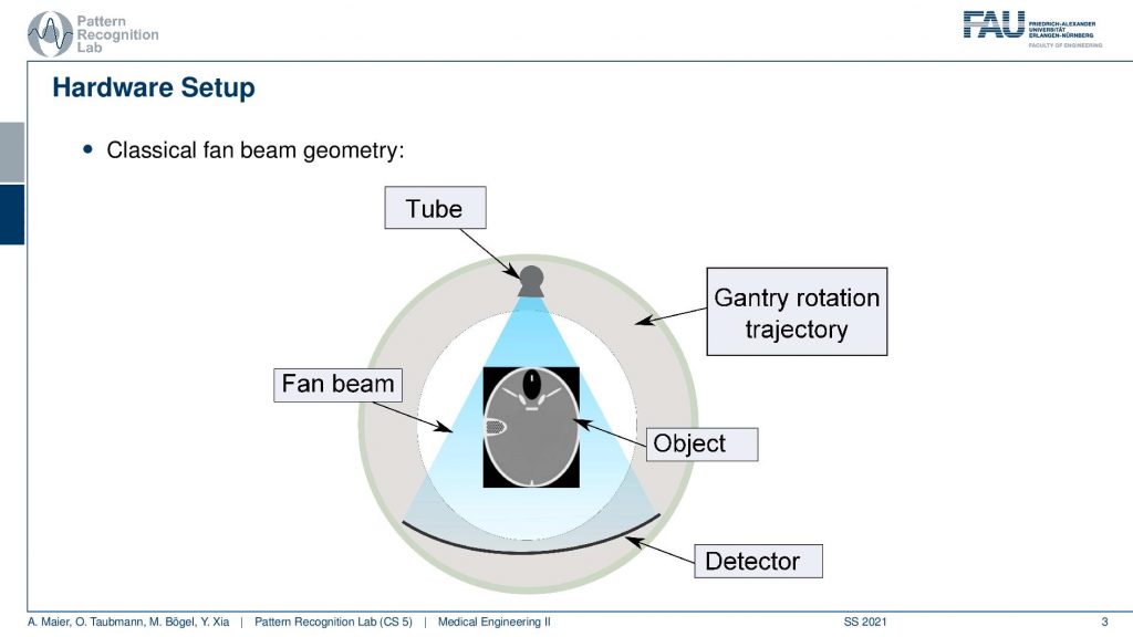
Now let’s review the CT measurement process. So what we typically have is a CT gentry like this one. You have a tube you have this banana-shaped kind of detector here and then you have the object in the center and we are acquiring this fan beam type of image. Now we rotate in order to get the entire reconstruction done and we rotate by at least 180 degrees plus this fan angle. If you want to make sure you go towards 360 degrees then you have measured all of the relevant rays. If we do this we have this sinogram that emerges.
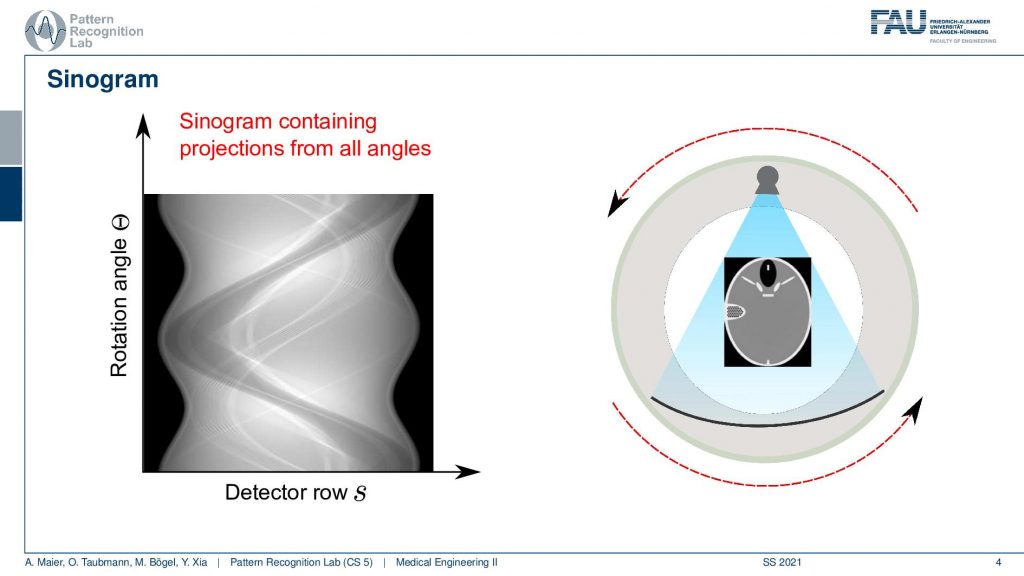
Here we essentially have the rotation angle and we have to detect the row and we see the objects that we have in the field of view. They get projected onto these sinusoid-like structures and from this, we can then reconstruct the actual image and the whole thing is obtained by rotation.
Now a key problem that we have is that we want to get the line integrals correctly. So far we have assumed that it is simply the sum of all the attenuation coefficients along the ray. What we essentially see is that one of these line integrals in one of the detector rows will just be one of these measurements and I repeat them for every detector index and this is exactly the integral over all the attenuation coefficients along this ray.
Now, this is the idealized kind of configuration. This led us to the idea that if this is the intensity at the source and then multiply it the exponential function minus the sum over the respective coefficients. You can then essentially solve this for the line integral by dividing over I0 taking the natural logarithm and the minus and then we get the line integral. So we’ve seen this before partially using a different notation but it doesn’t matter it’s the same concept. This is something that we have been assuming all the time.
But it’s not entirely correct because we have polychromatic x-rays. The problem here is that the actual x-rays are not mono-energetic but they form a continuous x-ray spectrum. So we have many energies and there is a different attenuation law actually in place than the simple Lambert-Beer. But we also have to integrate over all of the energies. So this can of course be fixed by using the beam hardening correction methods that we’ve seen previously. But obviously, it would be much better if we design our measurement process in a way that we can also intrinsically solve this problem.
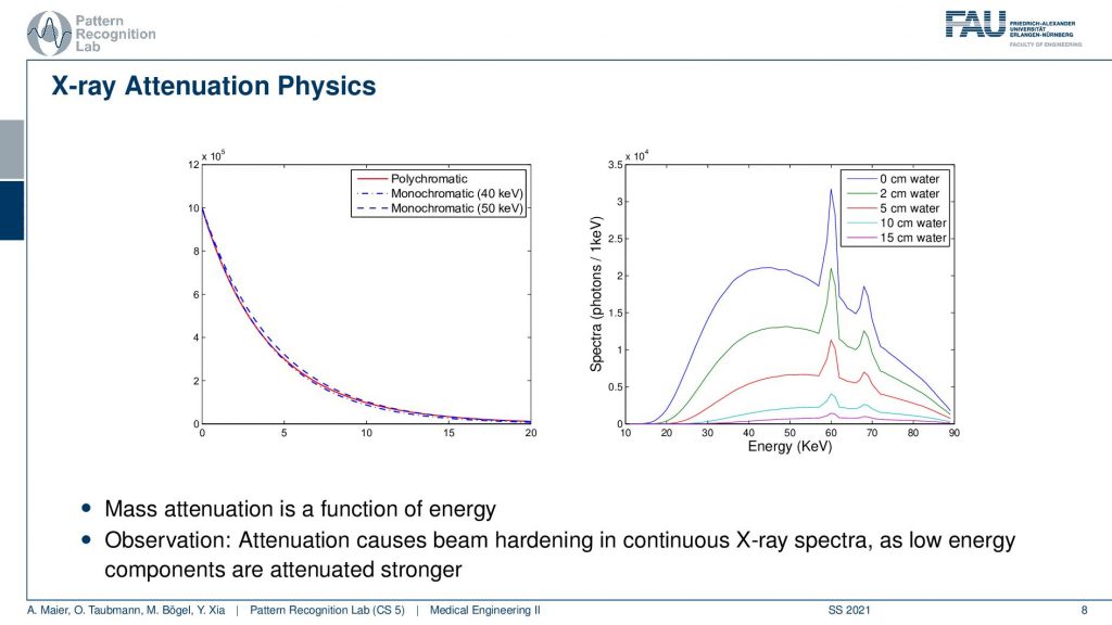
So what’s the problem? We’ve seen that if we have different acceleration voltages then we essentially get also different effects. What you see here on the right-hand side is the effect on the spectrum with different lengths of water on the path. You see the more water I have on the path, the more the shape of the spectrum is changing and in particular, its average energy is going up. So you’ve seen that before the more I increase the number of centimeters of water, the more the average energy in this kind of spectrum is increasing. So you see that the energy goes up and this is the reason for the beam hardening effect. You can then also see that if we have different materials then we don’t get essentially the absorption of a monochromatic behavior. So the monochromatic behavior would be the dashed lines here but we observe this polychromatic behavior which is a mixture of the two. Well, this is a problem and we’ve seen that it causes beam artifacts.
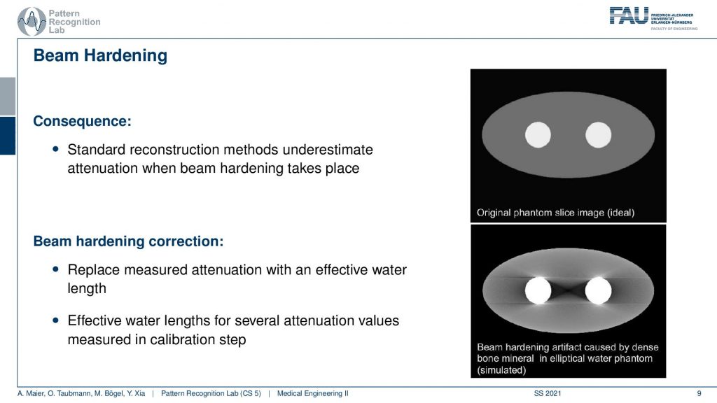
You see that we then get these streaking effects here in between and we’ve seen in the previous video that there’s also be more correction approaches that can help us with this. But we have to estimate and calibrate them and they’re very specific to the materials used. So if we have some new material showing up that we didn’t model in the beam hardening approach it may cause even more artifacts. So that’s not great. So we have to do something about that.
This brings us to the idea of spectral CT now in spectral CT the idea is not just to measure single energy or a single mixture of energies. But we want to have multiple of these measurements. So we kind of not just measure the attenuation but we measure the spectrum. So essentially the spectrum of energies of our photons. Then we can determine the spectral attenuation coefficient. So the energy-resolved attenuation coefficients. If we find a good way how to decompose them, then we should be able to figure out how much of a specific material has been on the path and we get rid of all the non-linearities that happened on the way.
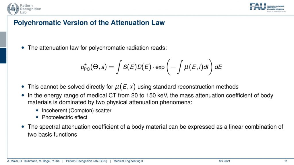
So this is actually what we have to deal with. This is the polychromatic absorption law and you see that what we previously had at the Lambert-Beer law is essentially this guy here. Now you see that there is a major difference. This μ is not just dependent on the l, but it’s also dependent on the E and the E is the energy that we have in the spectrum. So there is a complete integration over our spectrum here. In this notation, we even separate it into the x-ray spectrum S and then the detector efficiency for that particular energy dE on the detector side. We’ve seen that when we’re discussing x-rays that the detectors are sometimes more or less sensitive towards certain energies. So this can also be modeled but effectively you just multiply the two and they get then to the number of the observed energy in that particular detector energy cell. So this is the key difference. Now we’re modeling not just μ but we model μ energy-dependent. Then of course we want to vary the energy ranges to be able to resolve them. So this is something that we somehow have to implement that I can get multiple measurements over different energy bins. This would then allow us to resolve also different energies and there are possibly also different materials.
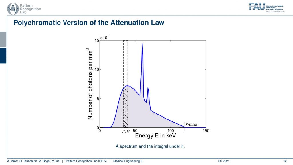
Now if we look at the polychromatic version visually what we compute with the spectral Lambert-Beer law is the area under the curve over this entire curve here. This is what our single detector element measures. So it measures the sum over all of these energies and in every individual energy the Lambert-Beer law holds with a different μ with a different x-ray attenuation coefficient. Now a spectral detector and would be able to get so-called energy bins and the smaller the energy bins are the closers I am to the actual Lambert-Beer monochromatic solution. Then I would only measure the integral within this energy bin here and then I can repeat that for several bins. Maybe if they’re equidistant, then I would get the next pin here and this way I would not just get single energy in the detector or, a single intensity that I observe, but I get that many channels. So if you think about the actual X-ray projection, then you see that this will be a projection with a specific intensity. But this one here will be also a specific projection. If I now add energies on top you see that I get another bin here and I get another projection. So I essentially get them different images of the scene that are sensitive to different energy ranges and wavelengths and you can already draw the similarity to human perception. So the human eye has three color channels which are red, green, and blue. With these three color channels, we can differentiate also certain properties of the materials. So it’s not just light intensity that we are perceiving but we can also figure out what kind of material is probably used and what the reflective properties are of the things that we’re looking at. This color is very important for our perception to figure out whether this is potentially dangerous or, not. So in X-rays, this is a little bit different but it also tells us material properties. So this is the idea of spectral CT. Now, this would be a detector solution. You will see to implement this is pretty hard. For measuring the different resolved energies, we have to do a couple of trade-offs to implement this.
So let’s look and how we can measure this.
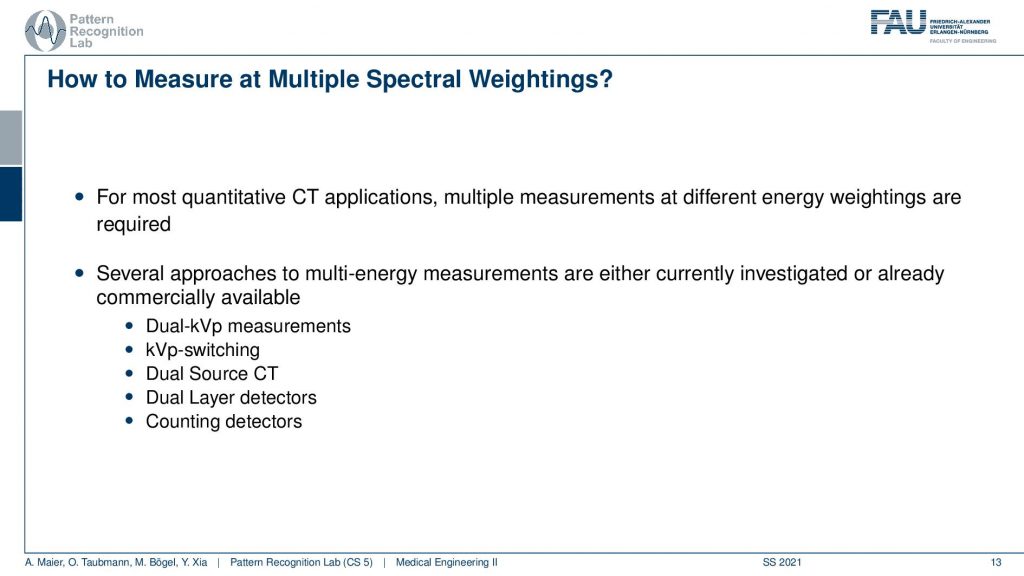
So how would we be able to measure these bins? We would like to make those small bins and just measure it the way how we can do that may be in an RGB camera but unfortunately, it’s not so easy. So we have to be able to create this spectral separation. This is the key factor that allows us the goodness of energy quantification. If we had many of these energy bins we would have a spectrum that is measured at every pixel. Key measurements or, key concepts to measure this are Dual-kVp measurements. So use two different spectra. You can switch very quickly in the spectra. You can use two sources and two detectors to get two different spectra. You can have dual-layer detectors and a very popular technique photon-counting detectors because they just count every individual photon and then they also assess the energy of this photon and then you can get these energy-resolved images. So these are the key technologies and we will have a look at them very quickly.
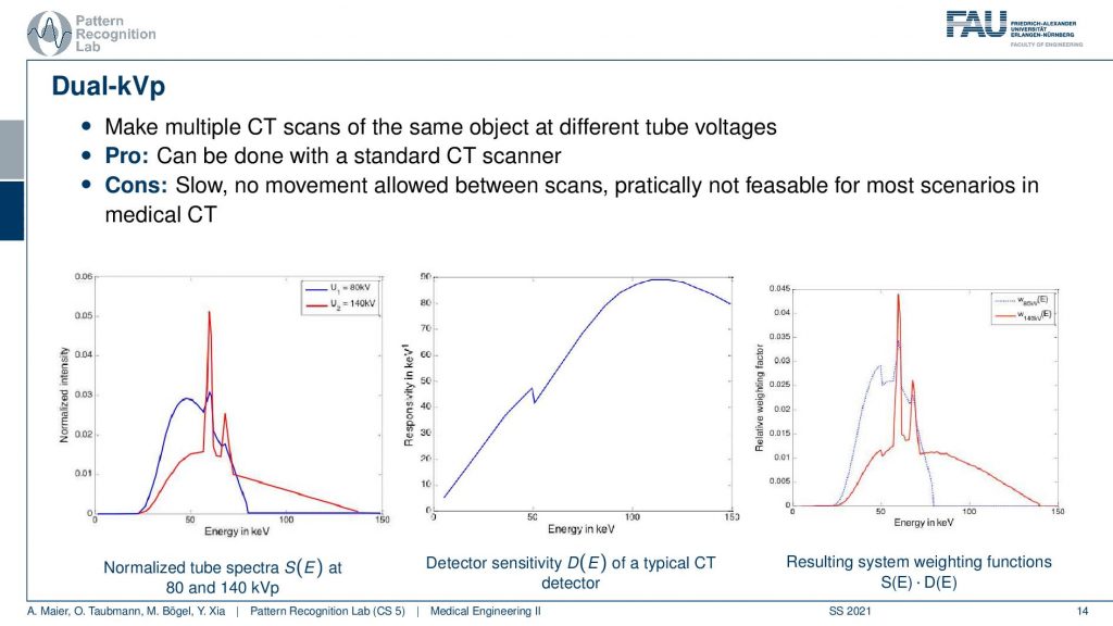
Dual-kVp means you do essentially two scans. So you scan the object once with the red spectrum here this is 140kV. Then you also scan it again with 80kV and you see here that we have this spectrum and we have this spectrum and this means we have measured two different weightings of the energies. Now previously we wanted to have something like this, right? We wanted to have these very neat energy bins and you see this has a huge overlap. So it’s not that great in terms of energy separation. But instead, I can maybe determine essentially this bin versus this bin here and you see that this is a mixture of the two spectra and the other bin is exclusively in the 140kV scan. So yeah this is not so great. You can separate them a little more if you also consider the detector sensitivity. Then you multiply the two and you see that the spectral separation is a little better. You can construct it in a way that at least the high energy bin is only concerning the high energy photons. But you see that in the low energy bin we’re able to only measure a mixture. So this is not so great. So if we have the first scan we essentially get the low energy part if we do the second scan with the 140kV we get a mixture of low and high energy. We then have to somehow disentangle the information in order to get the bins. So not that great but it’s one approach to do it. If you do it in repeated scans it’s slow because you have to scan twice. So that’s not that great.
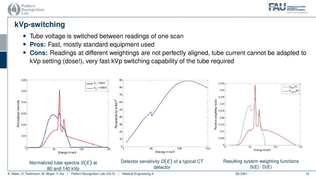
Well, another approach is called kVp-switching and this is for a tube that’s pulsed because there you have different x-ray pulses in every image. So what you can do is essentially over the rotations you can say okay I take a 140kV and an 80kV acquisition and I do an alternating acquisition of the two energies. This way I do just one rotation and from all view angles, I get essentially the 80 kV and the 140 kV situation. So this is better because we only have one rotation. But it also has a problem because the readings are at different positions. So I never observe the same line integrals because effectively I’m doing one projection from this angle and then I’m rotating. So the next projection will be taken from other angles. And I want to take the line integrals in order to disentangle information. This is lost here because I never observe the same line integrals. But I actually can only do a spectral resolution after reconstruction and then I have all the non-linearities in the reconstruction process. Also not that great but it can be used.
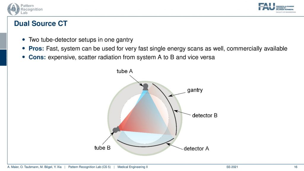
Well, what else? There is the dual-source. Now the dual-source is two tubes. So I have tube A and tube B and now I do them in two different energies. I do a single spin. So it’s fast but we have the problem that it’s expensive. We have to have two times the hardware and then there’s also scattered radiation that makes things hard. So it’s also not ideal but this way I can get at least the scans done in a very quick time. I also have the problem that the line integrals are not acquired at the same position. So it can be done to rebinning if you calibrate it well, you get close. So you can also work on a projection basis. But then there’s some interpolation involved but it does dual-energy and this is commercially available as a product and you can use it for material separation and it can be for example used to differentiate Calcium and Iodine. So you can differentiate whether in a certain voxel is a contrast agent or bone. So this is quite useful. It can also be used for scoring of the liver and stuff like that.
Another quite popular measurement concept is dual-layer detectors.
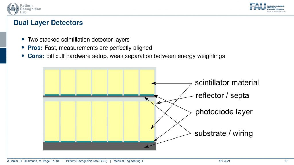
So here you have a detector and what’s better than one detector? Well, two detectors and two layers. The idea here is that if you have photons coming in then the lower energy ones will be absorbed here, while the higher energy ones will go through the first detector and then be detected here in the second detector. Now, this is a very nice principle. It can be constructed but you have a couple of problems. So first of all, you may have dual detection events that you detect this event here and here. So you somehow have to disentangle this. What can also happen is that the actual you know there’s the TFT array and the structure of the electronics here and there is metal in there and metal is not that great because X-rays are very sensitive to metal. This can also cause shadow images in the detector below. So it’s difficult to construct but it is a pretty good technique that would allow us to separate different energies. So there are some detectors of those available and they are also being used in research.
Now the prime category of detectors are the so-called photon counters and they follow the Optical counting. So they detect each photon individually. The cool thing is that if you detect one photon you can also essentially measure the energy of that photon because you know it’s just one photon and then by the height of the peak you know how high the energy was. This is then done with some kind of counting direct converters. What they do is they essentially then start counting with bins. So you have several energy bins and this is probably the closest to what we have with the kind of detectors that we showed earlier where we really have energy bins. Because for every photon we assign it to a bin and then this allows us maybe to two, three, or even four bin detectors that separate the energies. There are even more expensive detectors that can do spectral measurements per pixel. But first of all, they’re very expensive, and second, they typically have rather large pixels. So these kinds of detectors then really are able to measure complete X-ray spectra in a single shot. But they typically have much much larger pixels and therefore then these kinds of detectors are not that frequently used in medical applications, but more in the terms of material testing.
Pros: fast measurement, perfectly aligned
Cons: pile up
Too many events too many photons arriving at the same time and you won’t be able to differentiate anymore whether it was a single event or two or three events. So you can’t differentiate anymore. Was it just a single high energy event or was it three low energy events and this is called pile up and this is causing a major problem for the photon counting detectors. These are the different approaches.
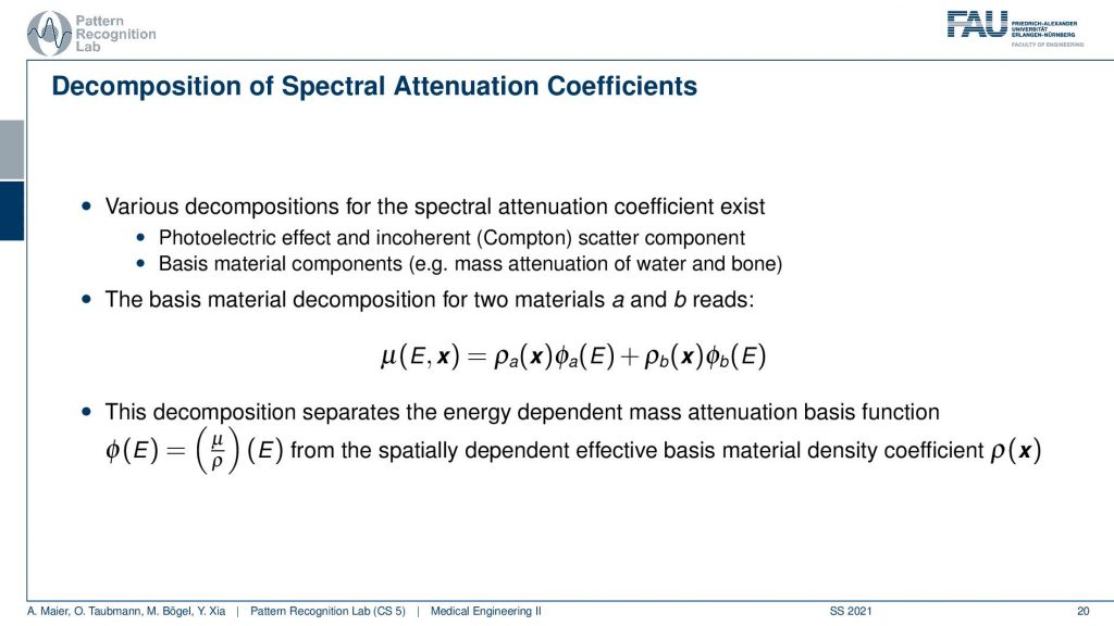
Then this allows us to build spectral kind of reconstruction algorithms. A key idea is that if I have now these different observations, then I can use them in order to differentiate the different physical effects. What do we do now? We have the energy-dependent observations at the detector. Then what we want to do is we want to figure out the actual source that causes the mismatch in the energies. One way to do it is that you project it onto a specific basis and it could be essentially coherent and a photoelectric effect scatter. So these are two kinds of sources that we can physically differentiate with or do basis material decompositions. So you try to find a kind of bases where you then assign a coefficient to like material path length and material is water and bone or, you take Compton-scatter and photoelectric effect and you measure the strength of this effect at that particular pixel. Once you did that you essentially get rid of the non-linearities and you can then reconstruct the water and bone components and this gives us basis materials. From the reconstructed basis images, we can then re-synthesize the same image at different voltages.
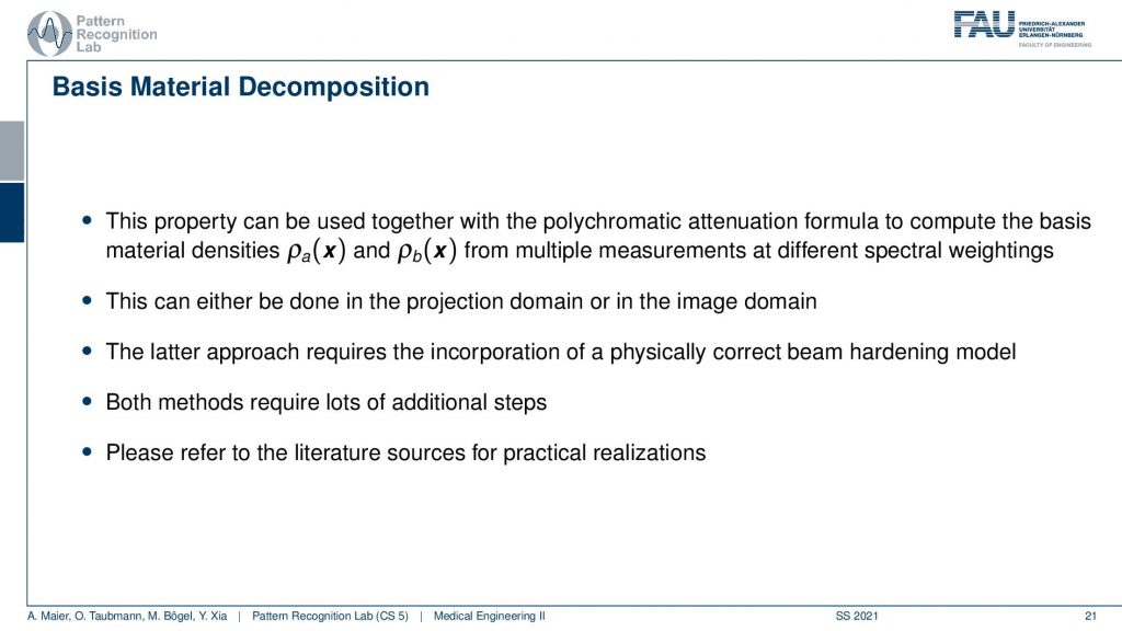
So this then gives rise to the idea of actually doing the spaces material decomposition and I have some examples here.
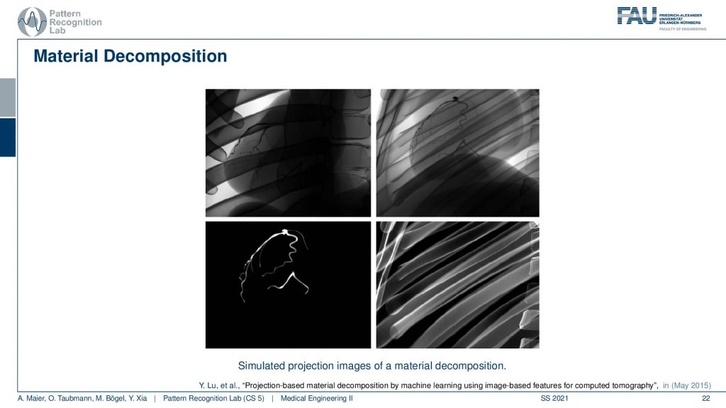
So you see that then we get different images for the materials. So you see the entire scene here on the top right and on the top left you see the same image in different energy. So this is a low-energy image. The right top is the high energy image and the left bottom is the iodine you see the iodine is only present in the coronary vessels. On the bottom right you see the bone image that only shows the ribs and this would be cool. I mean this is from a simulation right but let’s say I plug in this image and this image and then I reconstruct from the two these two basis images. So that would be cool and imagine if you could do that really well. Then you would be able to differentiate bones. So here they would only reflect the motion that is caused by the breathing and this image here would have superimposed the breathing motion and the heart motion. So this would be really cool for reconstruction because now I can disentangle different motions right. So unfortunately the material separation doesn’t work this well and this is only the actual ground truth. In the simulation, it works kind of well.
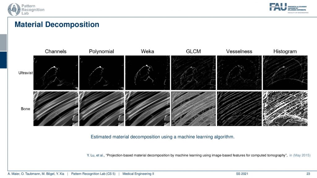
So you see if we do kind of deep learning-based approaches like here this built on Weka we get a pretty good separation. At least in the simulation, this works pretty well. Then if we have very simple approaches they completely fail in the construction and it doesn’t work only the physics-based model also works already pretty well. Well, this is for a simulation result. Unfortunately, if you go to a real detector then you get images like this one.
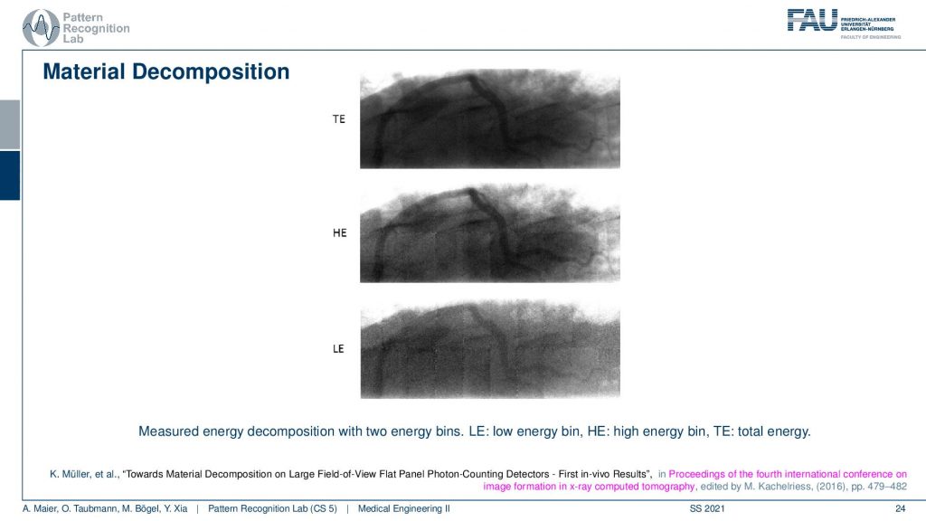
So the first one is the total energy. The second one is the high energy and the last one the low energy and you somehow see that there is a vessel here. You see this vessel. It’s here and now we know that these are different energies and we want to decompose them. Now, this is from an animal experiment with a very early study by K Mueller, and this was conducted actually in 2016. So a very early photon-counting detector.
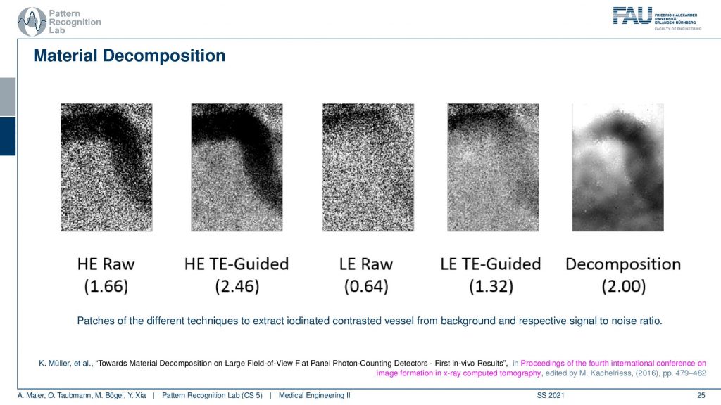
If you now look at the decomposition results it’s yeah so of course if we would have the high energy raw image. This is then an additional guided filter to get the actual noise a little bit down. This is the raw low energy image and then you already see there’s almost no contrast in the low energy image. You can denoise it a little bit so that it looks better. Then you can take this image and this image and decompose it into the contrast that is present and then you get an image like the last one. So this is the decomposition. This is actually the best decomposition we could get. What we figured out during those experiments is unfortunately the small detector. So first of all you see that we are only working on the small detector and the reason why working on the small detector is that the large detector is actually built from tiles of this size. If you have two neighboring tiles the energy separation is different. They don’t have the same thresholds, although you configure them in the same way. They have different thresholds for differentiating energy. So building one model for the entire system is not possible. So we only concentrated on the decomposition within one tile and you can already see that the thresholds within one tile are different. So you have a variation of the energy threshold that is constructing the bins between the actual detector pixels. This is a huge problem and caused a lot of artifacts. So with the very early prototype detectors, the material separation wasn’t that great. Still, I think it’s an exciting technology and you know this was 2016 and now we are already much more advanced of the technology. There are actually first photo counters available in clinical evaluation. So I think if we go back and revisit this, we could probably get much better decomposition results. Also, there is this huge advance with deep learning methods and artificial intelligence and they might be able to learn this energy dependence across the actual detector. So this is still exciting. This is a research result and yeah it didn’t get such nice results.
Obviously, you can also work with dual-energy scanners.
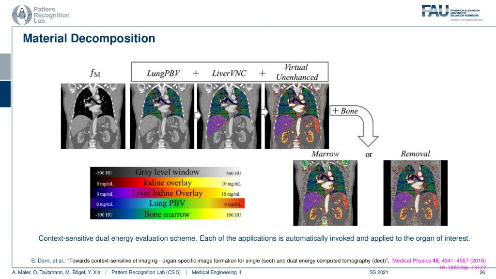
Then you can also do this and you may use prior knowledge in order to do the material decomposition. It is done in the work by Sabrina Dorn and was published here in medical physics. So what we can do is we can do a segmentation. So this is a kind of input image and then we segment the lung, the liver, and also other organs like the kidneys. Now we know the properties of the kidneys and depending on where you are in the body you can then use other materials for the material decomposition. This allows us then to get an analysis done for the lung and for the liver and the kidneys in a single scan. But we use essentially automatic segmentation methods to identify the relevant regions. In the relevant regions, we can then assume different materials because we know that in the lung we typically have these compounds, and in the liver, we have these compounds and then we can make a much better material separation and analysis compared to assuming the same model all over the body. Very well and interesting kind of application.
We have a couple of take-home messages. We explained today beam hardening and spectral CT and found out how we can actually pursue a base material decomposition. We looked into the different measurement approaches.

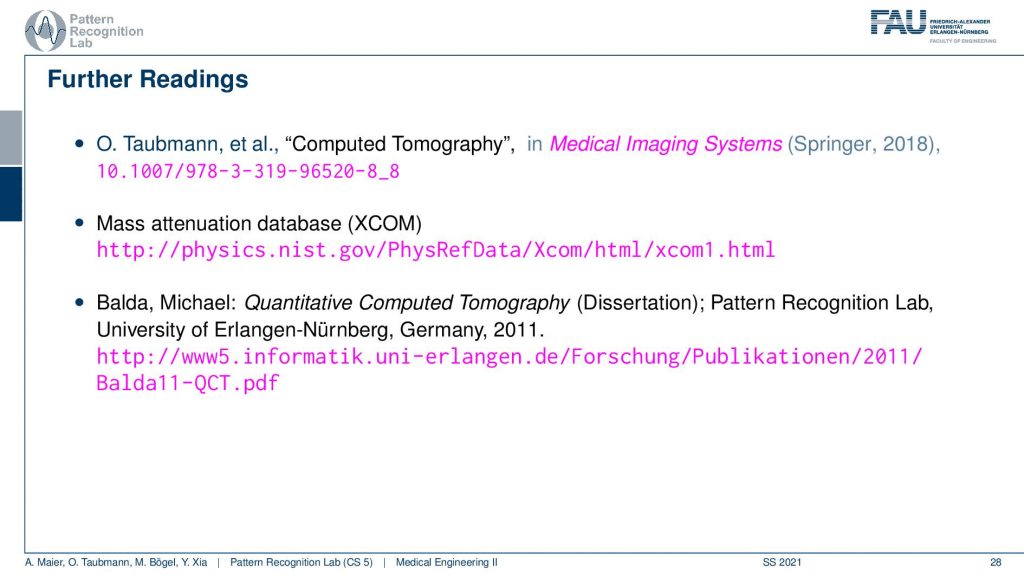
I have a couple of further readings in particular some of the papers that I referenced in the slides are here but you have to go back to the slides to see all of the references. In particular, if you’re interested in these things there’s of course, our book chapter which is very good by Oliver Taubman. What is very important is the Mass Attenuation Database. This is cool. This is the physics department of the National Institute of Standards and Technology. They have reference values for all kinds of materials. So for all elements and all frequent compounds, they have the reference values available downloadable for free and you can then supply them to your simulation and figure out how they actually match your kind of experiments. Also, what I can recommend we had a very good Ph.D. thesis by Michael Balder on Quantitative Computed Tomography. It was a very nice dissertation and he was one of the first to investigate these quantitative and spectral reconstruction algorithms. I can definitely recommend reading his thesis if you’re more interested in these topics.
Okay, so this already brings us to the end of this video. So now you know about X-rays, you’ve seen how to reconstruct. You’ve seen the reconstruction algorithm. You’ve seen the artifacts and the design specs and how to determine the resolution of the systems and so on. Now you’ve already seen how we can deal with the polychromatic effects that happen in the X-rays on a rather coarse level. But you see that we can actually harness this information in order to differentiate the different materials. So that’s pretty cool and yeah there’s a little bit more about x-rays that I would like to show to you. This is a rather experimental kind of setup. It’s called face contrast imaging and it is actually using the wave properties of X-rays and there we can not just reconstruct the absorption but also the phase of the signal. You’ll see that this is actually a rather early technology. Most of this is experimental, but still, I would like to highlight this because it very nicely fits into our setup with the different modalities from in clinical use already up to highly experimental but potential game-changers of the future. So thank you very much for watching and I’m very much looking forward to seeing you in the next video. Bye-bye!!
If you liked this post, you can find more essays here, more educational material on Machine Learning here, or have a look at our Deep Learning Lecture. I would also appreciate a follow on YouTube, Twitter, Facebook, or LinkedIn in case you want to be informed about more essays, videos, and research in the future. This article is released under the Creative Commons 4.0 Attribution License and can be reprinted and modified if referenced. If you are interested in generating transcripts from video lectures try AutoBlog
References
- Maier, A., Steidl, S., Christlein, V., Hornegger, J. Medical Imaging Systems – An Introductory Guide, Springer, Cham, 2018, ISBN 978-3-319-96520-8, Open Access at Springer Link
Video References
- Andreas Maier – X-ray Material Decomposition https://youtu.be/XGXpIX8gPWc
- Dual Source CT – Fast Temporal Resolution https://youtu.be/oR7DwWzMZRs