
Attention Mechanisms
These are the lecture notes for FAU’s YouTube Lecture “Deep Learning“. This is a full transcript of the lecture video & matching slides. We hope, you enjoy this as much as the videos. Of course, this transcript was created with deep learning techniques largely automatically and only minor manual modifications were performed. Try it yourself! If you spot mistakes, please let us know!
Welcome back to deep learning! Today, I want to tell you a bit about attention mechanisms and how they can be employed in order to build better deep neural networks. Okay, so let’s focus your attention on attention and attention mechanisms.
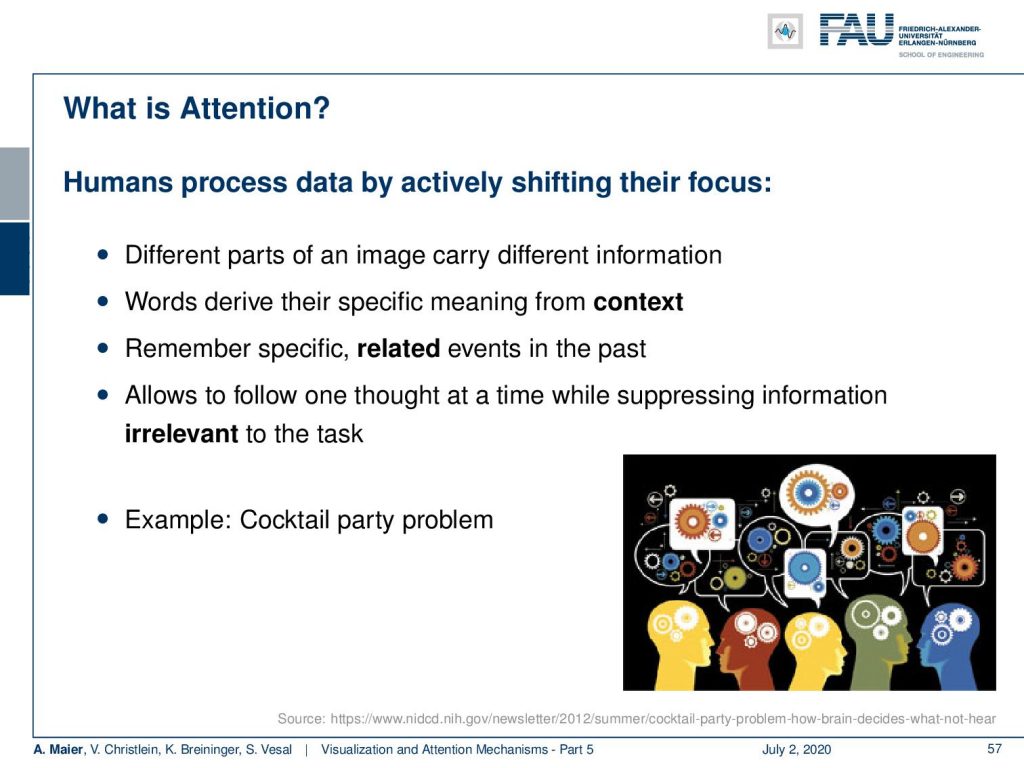
So, what is attention? Well, you see that humans process data actively by shifting our focus. So, we can focus on specific parts of the images because they carry different information. Of course, for some words, for example, we can derive the correct meaning only by means of context. Therefore, you want to shift your attention, and the way how you shift your attention may also change the interpretation. So, you want to remember specific related events in the past in order to influence a certain decision. This then allows us to follow one part at a time while suppressing information irrelevant for the task. So, this is the idea: You only want to focus on the relevant information. One example that you could think of is the cocktail party problem. We have many different people talking and you just focus on one person. By specific means like by looking at the lips of that person, you can focus your attention on lips. Then you can also kind of use your stereo hearing as a kind of beam-former to only listen to that particular direction. Doing so, you’re able to concentrate only on a single person, the person that you were talking to using this kind of attention mechanism. We do that quite successfully because otherwise, we would be completely incapable of communicating a cocktail party.
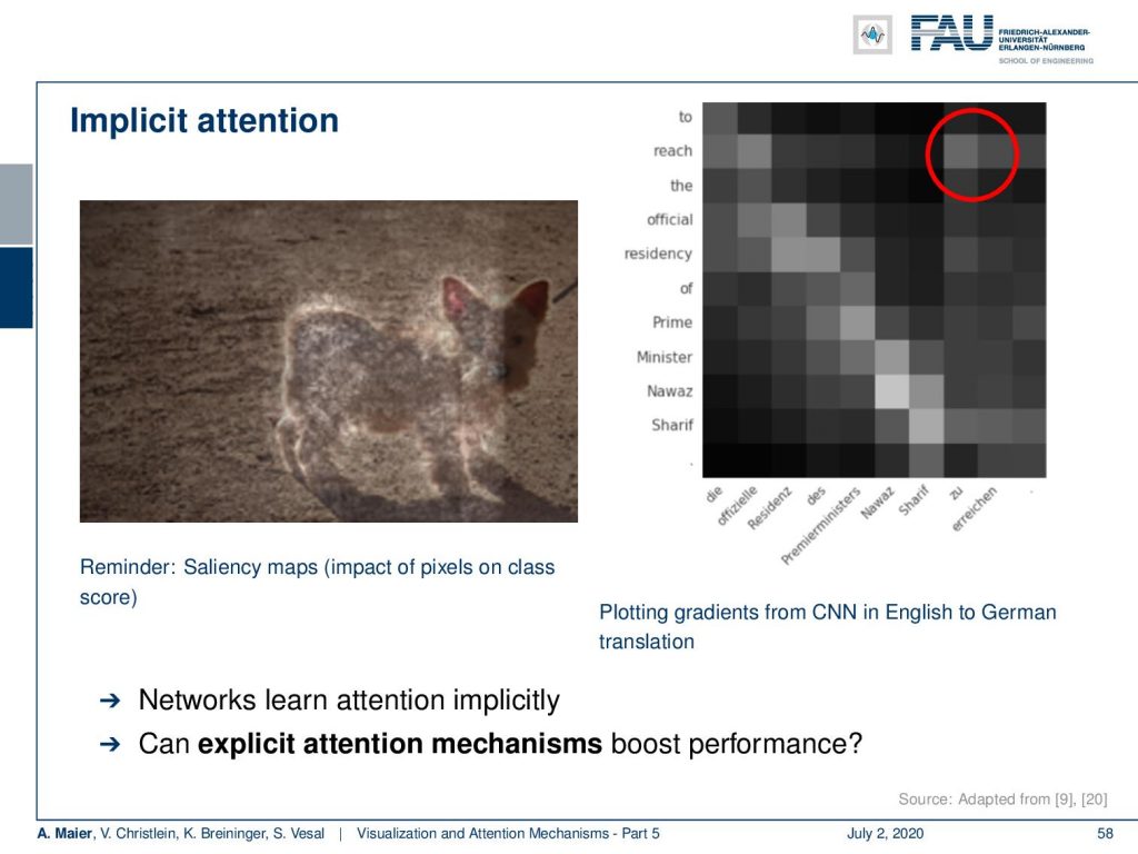
So what is the idea? Well, you’ve already seen those salience in maps. You could argue that we only want to look at the pixels that are relevant to our decision. In order to make the decision, in fact, we will start not with images, but we want to talk first about the sequence to sequence models. Here, you can see a visualization of gradients from a CNN type of model that is used to translate from English to German if you now start plotting those gradients. So, this is essentially the visualization technique that we already looked at in image processing. You can now see the gradient with respect to that particular input of the respective output. If you do so, you can notice that in most cases, you see this essentially a linear relationship. English and German have of course very similar sequences in terms of words. Then you see that the actual beginning of the sequence which starts with “to reach the official residency of Prime Minister Nawaz Sharif” is then translated to “die offizielle Residenz des Premierministers Nawaz Sharif zu erreichen”. So, “zu erreichen” is “to reach” but “to reach” is first in English and it goes last in German. So, there’s a long temporal context between the two. These two words essentially translate to those two. So, we can use this information that we can generate with gradient backpropagation in order to figure out which parts of the input sequence are related to which parts of the output sequence. Now, the question is how can we use this in order to boost the performance.
Let’s look at a typical translation model. So, what is typically done in sequence the sequence models if you work with recurrent neural networks? What you do is you have a forward-pass in an encoder network. This receives an input sequence. From the input sequence, as we discussed earlier, we can compute the hidden States h subscript 1 to h subscript T. So, we have to process the entire sequence in order to compute h subscript T. Then, h subscript T is used as a context vector for the decoder network. So, h subscript T is essentially the representation of the state or the actual meaning of this sentence. Then, h subscript T is decoded into a new sequence by the decoder network. Then this generates a new sequence of own hidden states that are s subscript 1 to s subscript T’. So note that the output, of course, can be of different lengths. So, we have two different strings of T and T’. This also generates an output sequence y subscript 1 to y subscript T’. So, this allows us to model different lengths in input and output, of course, you may have a different number of words in two different languages.
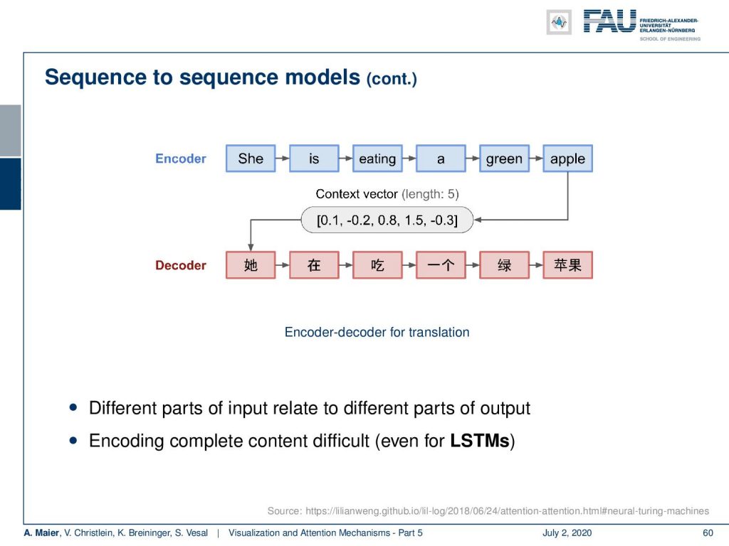
So, now when we actually do this decoding. Then, you see that we have to encode everything into this context vector and this encoding may be very difficult because we have to encode the entire meaning of the sentence into one context vector. This may also be very difficult even for LSTMs.
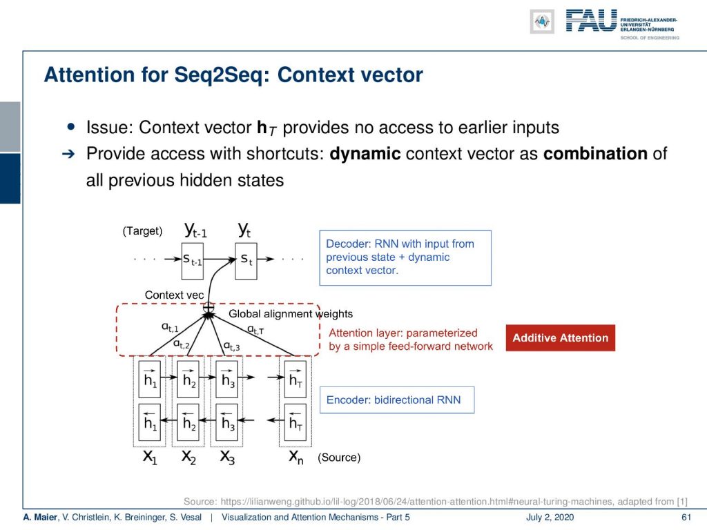
So, the idea is now to introduce attention. Attention for sequence-to-sequence modeling can be done with a dynamic context vector. The idea is now that we have this context vector h subscript t. The issue that we had is this context vector h subscript T and it does not allow any access to earlier inputs because it was only obtained at the very end of the sequence. So, the idea now is to provide access to all contexts using a dynamic context vector as a combination of all previous hidden states.
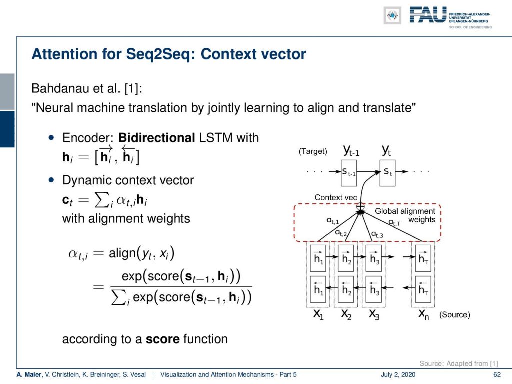
So here, we see a bi-directional RNN which does one encoding by a forward-pass. So, you start with x subscript 1 and create a hidden state 1 and go to x2 and so on. Then, you run exactly the opposite sequence. So, you start with x subscript n and go to x subscript (n-1) to create another context vector which is exactly from the backward processing of the same input sequence. This then gives you access to several hidden states and those hidden states, we can essentially concatenate from the two passes. With those hidden states, we then want to do a linear combination with some combination weights α. So, this is a weighted average of the different hidden states. So, we multiply them with the respective α add them up and provide this as an additional dynamic context for our decoder RNN. So, the idea is that we want to generate these weights α using a dynamic procedure.
Okay. So, let’s look at how we can actually compute those α’s. The idea that is presented in [1] is that you essentially try to produce alignment weights. So, if the state is relevant for the current observation in the decoding, then you wanted to get a high score. If the state is not so relevant, then you want to give it a low score. So, the α’s encode the relevance of the current state with respect to the currently produced output. Now, you may argue “Okay. So, how can I actually generate this score?” So, of course, we can put it into some softmax function. Then, they will be scaled between 0 and 1. So, that solves the problem. So, we can produce any kind of measurement of similarity and we can actually propose different approaches.
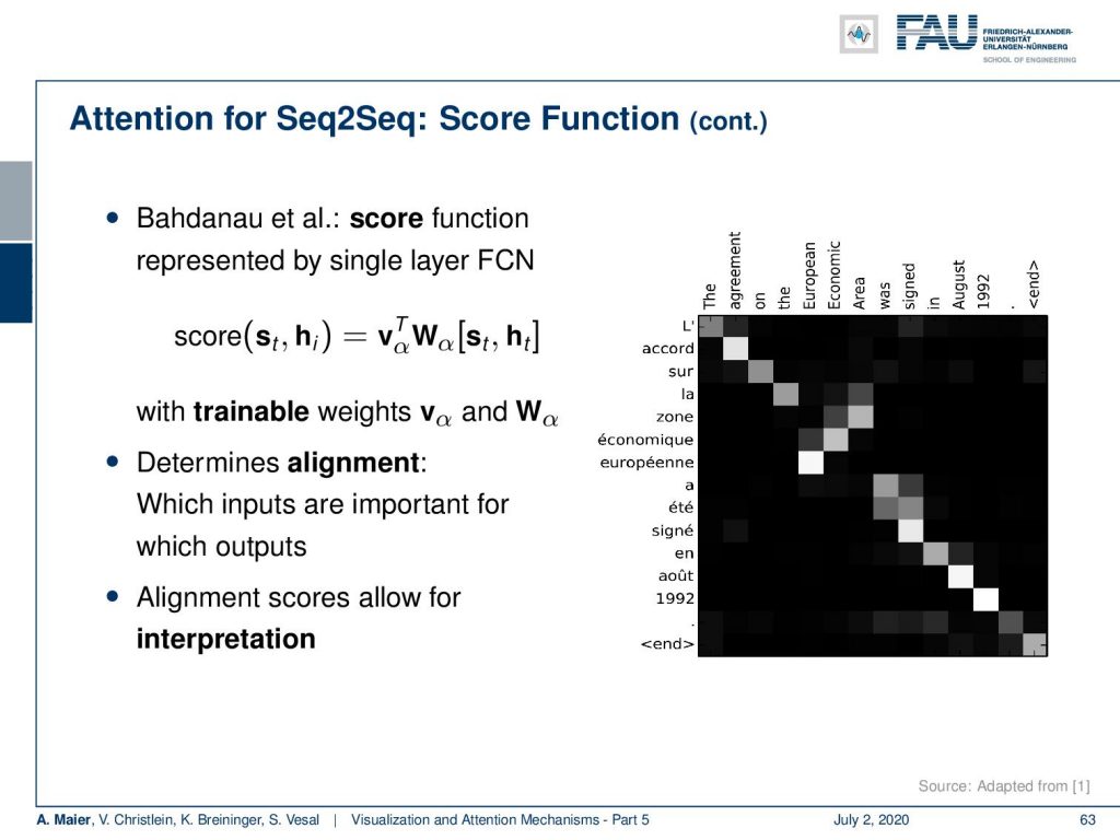
What they propose in [1] is actually to a score function. Now, the score function is represented by a matrix W subscript α and an additional vector v subscript α. These two are simply trainable. So we essentially use this property of universal function approximation that we don’t have to set the score function but instead, we simply train it. So it determines the ideal alignment which inputs are important for which outputs. The nice thing is, that you can also visualize those weights for specific inputs. So, it allows also interpretation by looking at the scores. We’re doing this here on the right-hand side example. This is again a translation setup where we want to translate from English to French. You can see that now these alignments essentially form a line. But there is one exception. So you see that the “European Economic Area” is decoded into the “zone economique européenne”. So, you can see that there is an inversion of the sequence and this inversion of the sequence is also captured in the attention by the alignment scores. So, this is a very good way of how to compute the score function.
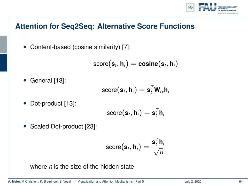
There are different alternatives. For example, in [7], they have simply the cosine between the two states to form the score. You could have a generalized inner product using some weight matrix W subscript α, you could have a dot product which is essentially just the correlation between the two states, and then you could also have a scaled dot product that somehow also respects the size of the hidden state. So, all of these have been explored and, of course, this depends on your purpose, what you’re actually computing. But you can see that we are essentially trying to learn a comparison function that tells us which state is compatible with which other states.
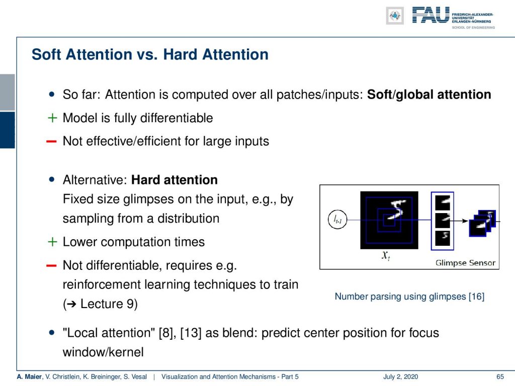
Ok. There are different kinds of attention. There’s soft attention versus hard attention. So, far we essentially had soft/global attention which is fully differentiable. But it’s not very efficient for large inputs. You can alleviate that by hard attention. Here, you fix on glimpses of the input. So, you take out small patches for example from images and sample this from a distribution. This, of course, implies much lower computation times. But the sampling process is unfortunately not differentiable. Then, you will have to look into other training techniques such as reinforcement learning to be able to train this. This has a much higher computing time. So, this is a certain drawback of hard attention. There are also things like local attention that is a kind of blend where you predict the center position for the focus and window or kernel. So, let’s see what we can do with that.
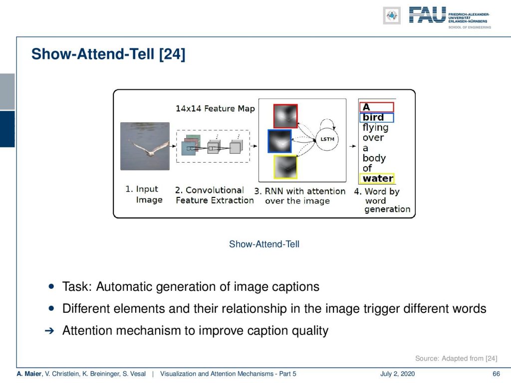
You can even do things like combining attention with image recognition. There’s a paper [24] that’s called show-attend-tell. It actually has the idea that you want to have an automatic generation of image captions. The different elements in their relationship in the image trigger different words. So, this means that the attention mechanism is used to improve the caption quality. How does this work? Well, you can see here now that we can compute the attention of a specific word.
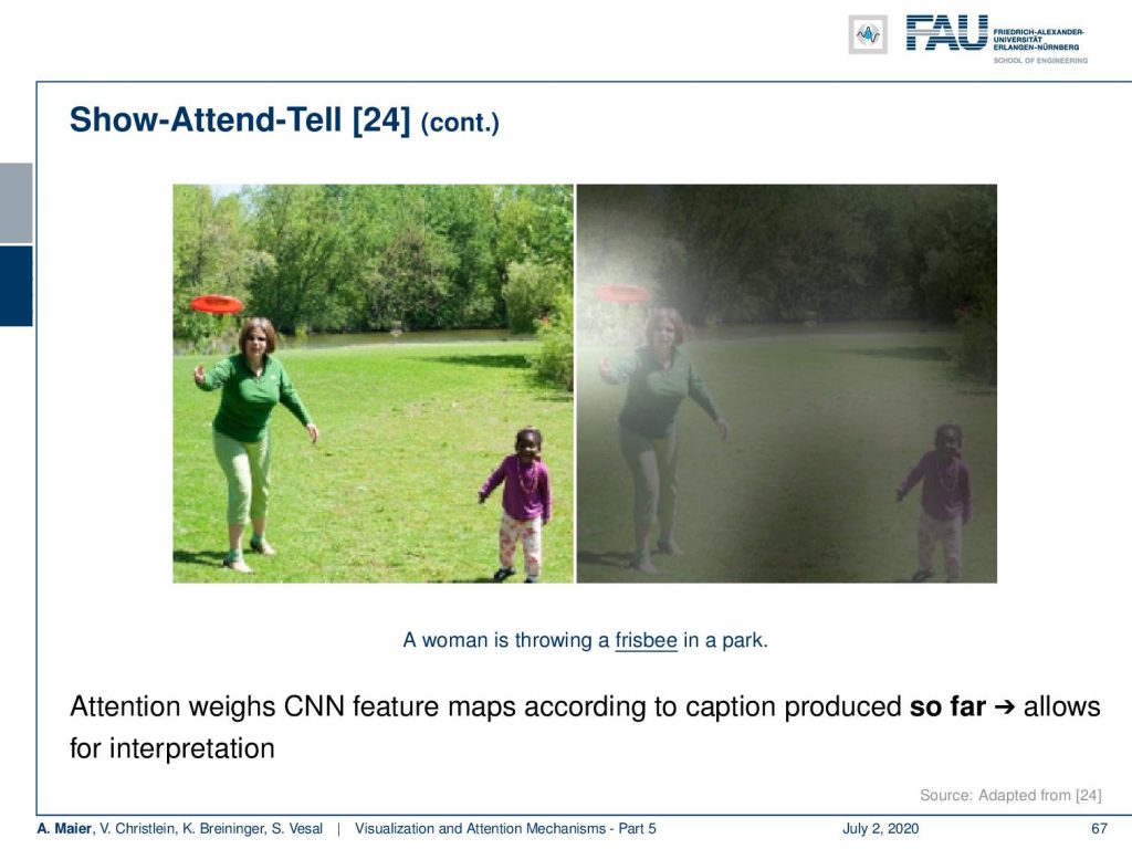
Here, you see that the sentence that was generated is “A woman is throwing a frisbee in the park”. Now, we can relate the frisbee with this attention map and you can see that we are actually localizing the frisbee in the image. So, this is actually a very nice way of using the CNN feature maps to focus the attention for their respective decoding at the respective position.
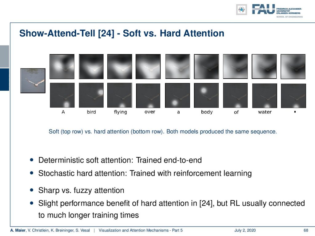
Here’s a comparison between soft and hard attention. You can see that the attention maps that are produced softly, they are fuzzier and are not as localized while the hard attention looks at only small patches. That’s the way how we designed it, but both of these techniques allow us to generate better image descriptions. Deterministic soft attention can be trained end-to-end. Well, for hard attention, we have to train using reinforcement learning. [24] shows that both attention mechanisms generate the same sequence of words. So, it’s actually working quite well and you have this side product that you can now also localize things in the image. Very interesting approach!
You can also expand this by something that is called “self-attention”. So, here the idea is to compute the attention of the sequence to itself. So, the problem that we want to tackle here is that if you have some input like “The animal didn’t cross the street because it was too tired.”, then we would like to know whether “it” refers to “animal” or “the street”. Now, the idea is that you want to enrich the representation of the tokens with context information. Of course, this is an important technique for machine-reading, question answering, reasoning, and so on so. We have an example sequence here: “The FBI is chasing a criminal on the run.” Now, what we do is we compute the attention of the sequence with respect to itself. This allows us to relate every word of the input to other words of the input. So, we can generate this self-attention.
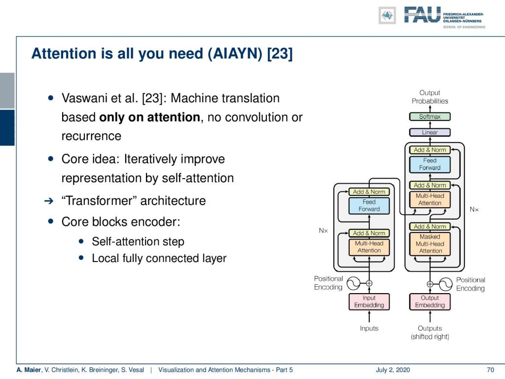
Why is this useful? Well, you can see that you can then also use this for machine translation. The network that they propose is only based on attention. So, there’s no convolutions and there is no recurrence for machine translation. So, attention is all you need. The core idea is now to iteratively improve the representation by this self-attention mechanism. This then gives rise to a kind of transformer architecture. It has two core blocks and the encoder, this is the self attention step, and the local fully connected layer which is then used to merge the different attention heads.
So let’s look at them in a little more detail. Of course, you need an encoder. We’ve already seen that for words, we can for example use one-hot-encoding. This is a very coarse kind of representation. So, this attention is all you need network learns an embedding algorithm. So, a general function approximator is used to produce an embedding that is somehow compressing the input. Then, it computes self-attention for each token. So, you could argue that you have a query token, a key which is a description for the query, and you produce a value for potential information. They are generated using trainable weights. Then, the alignment between query and key is a scaled dot product that determines the influence of the elements in v. So, we can express this as softmax of the outer product of q and k and this is then multiplied to the vector v to produce the attention value.
Now with this attention, we actually have a multi-head-attention. So, we don’t just compute a single attention, but different versions of the attention per token. This is used to represent different subspaces. Then, this local per token information is recombined using a fully connected layer. This is then stacked and using several attention blocks in [23]. So, this allows a step-by-step context integration. They have an additional positioner encoding to represent the word order. So, this is now at the input embedding. Now, if you look at the decoder it follows essentially the same concept as the encoder. There’s an additional input/output attention step and the self-attention is only computed on previous outputs.
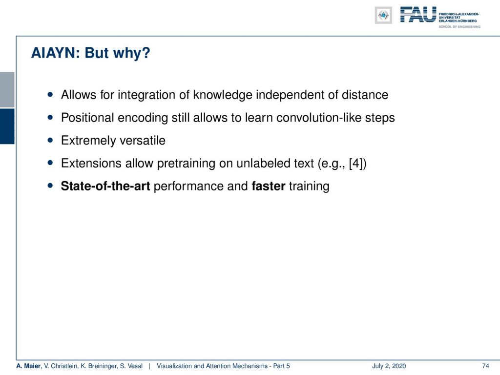
You could argue why do we want to do that? Well, it allows for an integration of knowledge independent of the distance. This positional encoding still allows us to learn convolution like steps. It is extremely versatile and extensions even allow pre-training using unlabeled text as you see in [4]. So reference for is the so-called BERT system. BERT is generated completely from unlabeled texts by predicting essentially the text sequence. The BERT embeddings have been shown to be extremely powerful for many different natural language processing tasks. A really popular system in order to generate unsupervised feature representation in natural language processing. These systems then have state-of-the-art performance and much faster training times.
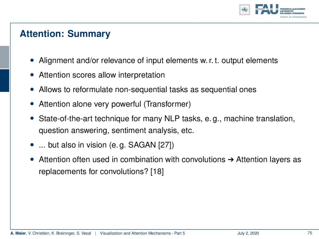
Okay. So, let’s summarize attention a bit. Attention is based on the idea that you want to align or find out the relevance of input elements with respect to specific output elements. The attention scores allow interpretation. It allows us to reformulate non-sequential tasks as sequential ones. The attention alone is very powerful because it’s a transformer mechanism. State-of-the-art techniques for many, many natural language processing tasks involve these attention mechanisms. It’s very popular for machine translation, question answering, sentiment analysis, and the like. But it also has been applied to vision, for example, in [27]. Of course, attention is also used in combination with convolutions but there’s also the question of whether attention layers can be seen also as a replacement for convolutions as shown in [18].
Okay. So, next time in deep learning, what’s coming up? Well, coming up is deep reinforcement learning! A really cool technique. We will have a couple of videos on this and we want to really show you this paradigm. How to produce a superhuman performance for playing certain games. So, the strategy is that we want to train agents that can solve specific tasks in a specific environment. We will show you an algorithm to determine a game strategy from playing the game itself. Here, the neural networks are moving beyond perception to really make decisions. If you watch the next couple of videos, you will also get instructions, how to finally beat all your friends in ATARI games. We will also show you a recipe to beat every human in go. So, stay tuned, stay with us. Watch the next couple of videos.
If you want to prepare for the exam with us, it would be good to look at the following questions: Why is visualization important? Something that everybody should know is “What is an adversarial example?”. Also, you should be able to describe the techniques that are used. Gradient-based techniques for visualization, optimization-based techniques, inceptionism, and inversion techniques. Why is it not safe to cut off your network after layer three and only keep the activations? Well, of course, they can be inverted if you know the network architecture. So, it may not be safe and anonymous if you store activations. We have some links to further readings. In particular, the deep visualization toolbox is really useful. In particular, if you want to learn a bit more about the attention techniques that we kind of very coarsely only covered in this video, there’s much more to say about this. But then we would have to go really deep into sequence modeling and machine translation which we can’t cover in this detail in this class. So, thank you very much for listening and hope to see you in the next video. Bye-bye.
If you liked this post, you can find more essays here, more educational material on Machine Learning here, or have a look at our Deep LearningLecture. I would also appreciate a follow on YouTube, Twitter, Facebook, or LinkedIn in case you want to be informed about more essays, videos, and research in the future. This article is released under the Creative Commons 4.0 Attribution License and can be reprinted and modified if referenced. If you are interested in generating transcripts from video lectures try AutoBlog.
Links
Yosinski et al.: Deep Visualization Toolbox
Olah et al.: Feature Visualization
Adam Harley: MNIST Demo
References
[1] Dzmitry Bahdanau, Kyunghyun Cho, and Yoshua Bengio. “Neural Machine Translation by Jointly Learning to Align and Translate”. In: 3rd International Conference on Learning Representations, ICLR 2015, San Diego, 2015.
[2] T. B. Brown, D. Mané, A. Roy, et al. “Adversarial Patch”. In: ArXiv e-prints (Dec. 2017). arXiv: 1712.09665 [cs.CV].
[3] Jianpeng Cheng, Li Dong, and Mirella Lapata. “Long Short-Term Memory-Networks for Machine Reading”. In: CoRR abs/1601.06733 (2016). arXiv: 1601.06733.
[4] Jacob Devlin, Ming-Wei Chang, Kenton Lee, et al. “BERT: Pre-training of Deep Bidirectional Transformers for Language Understanding”. In: CoRR abs/1810.04805 (2018). arXiv: 1810.04805.
[5] Neil Frazer. Neural Network Follies. 1998. URL: https://neil.fraser.name/writing/tank/ (visited on 01/07/2018).
[6] Ross B. Girshick, Jeff Donahue, Trevor Darrell, et al. “Rich feature hierarchies for accurate object detection and semantic segmentation”. In: CoRR abs/1311.2524 (2013). arXiv: 1311.2524.
[7] Alex Graves, Greg Wayne, and Ivo Danihelka. “Neural Turing Machines”. In: CoRR abs/1410.5401 (2014). arXiv: 1410.5401.
[8] Karol Gregor, Ivo Danihelka, Alex Graves, et al. “DRAW: A Recurrent Neural Network For Image Generation”. In: Proceedings of the 32nd International Conference on Machine Learning. Vol. 37. Proceedings of Machine Learning Research. Lille, France: PMLR, July 2015, pp. 1462–1471.
[9] Nal Kalchbrenner, Lasse Espeholt, Karen Simonyan, et al. “Neural Machine Translation in Linear Time”. In: CoRR abs/1610.10099 (2016). arXiv: 1610.10099.
[10] L. N. Kanal and N. C. Randall. “Recognition System Design by Statistical Analysis”. In: Proceedings of the 1964 19th ACM National Conference. ACM ’64. New York, NY, USA: ACM, 1964, pp. 42.501–42.5020.
[11] Andrej Karpathy. t-SNE visualization of CNN codes. URL: http://cs.stanford.edu/people/karpathy/cnnembed/ (visited on 01/07/2018).
[12] Alex Krizhevsky, Ilya Sutskever, and Geoffrey E Hinton. “ImageNet Classification with Deep Convolutional Neural Networks”. In: Advances In Neural Information Processing Systems 25. Curran Associates, Inc., 2012, pp. 1097–1105. arXiv: 1102.0183.
[13] Thang Luong, Hieu Pham, and Christopher D. Manning. “Effective Approaches to Attention-based Neural Machine Translation”. In: Proceedings of the 2015 Conference on Empirical Methods in Natural Language Lisbon, Portugal: Association for Computational Linguistics, Sept. 2015, pp. 1412–1421.
[14] A. Mahendran and A. Vedaldi. “Understanding deep image representations by inverting them”. In: 2015 IEEE Conference on Computer Vision and Pattern Recognition (CVPR). June 2015, pp. 5188–5196.
[15] Andreas Maier, Stefan Wenhardt, Tino Haderlein, et al. “A Microphone-independent Visualization Technique for Speech Disorders”. In: Proceedings of the 10th Annual Conference of the International Speech Communication Brighton, England, 2009, pp. 951–954.
[16] Volodymyr Mnih, Nicolas Heess, Alex Graves, et al. “Recurrent Models of Visual Attention”. In: CoRR abs/1406.6247 (2014). arXiv: 1406.6247.
[17] Chris Olah, Alexander Mordvintsev, and Ludwig Schubert. “Feature Visualization”. In: Distill (2017). https://distill.pub/2017/feature-visualization.
[18] Prajit Ramachandran, Niki Parmar, Ashish Vaswani, et al. “Stand-Alone Self-Attention in Vision Models”. In: arXiv e-prints, arXiv:1906.05909 (June 2019), arXiv:1906.05909. arXiv: 1906.05909 [cs.CV].
[19] Mahmood Sharif, Sruti Bhagavatula, Lujo Bauer, et al. “Accessorize to a Crime: Real and Stealthy Attacks on State-of-the-Art Face Recognition”. In: Proceedings of the 2016 ACM SIGSAC Conference on Computer and Communications CCS ’16. Vienna, Austria: ACM, 2016, pp. 1528–1540. A.
[20] K. Simonyan, A. Vedaldi, and A. Zisserman. “Deep Inside Convolutional Networks: Visualising Image Classification Models and Saliency Maps”. In: International Conference on Learning Representations (ICLR) (workshop track). 2014.
[21] J.T. Springenberg, A. Dosovitskiy, T. Brox, et al. “Striving for Simplicity: The All Convolutional Net”. In: International Conference on Learning Representations (ICRL) (workshop track). 2015.
[22] Dmitry Ulyanov, Andrea Vedaldi, and Victor S. Lempitsky. “Deep Image Prior”. In: CoRR abs/1711.10925 (2017). arXiv: 1711.10925.
[23] Ashish Vaswani, Noam Shazeer, Niki Parmar, et al. “Attention Is All You Need”. In: CoRR abs/1706.03762 (2017). arXiv: 1706.03762.
[24] Kelvin Xu, Jimmy Ba, Ryan Kiros, et al. “Show, Attend and Tell: Neural Image Caption Generation with Visual Attention”. In: CoRR abs/1502.03044 (2015). arXiv: 1502.03044.
[25] Jason Yosinski, Jeff Clune, Anh Mai Nguyen, et al. “Understanding Neural Networks Through Deep Visualization”. In: CoRR abs/1506.06579 (2015). arXiv: 1506.06579.
[26] Matthew D. Zeiler and Rob Fergus. “Visualizing and Understanding Convolutional Networks”. In: Computer Vision – ECCV 2014: 13th European Conference, Zurich, Switzerland, Cham: Springer International Publishing, 2014, pp. 818–833.
[27] Han Zhang, Ian Goodfellow, Dimitris Metaxas, et al. “Self-Attention Generative Adversarial Networks”. In: Proceedings of the 36th International Conference on Machine Learning. Vol. 97. Proceedings of Machine Learning Research. Long Beach, California, USA: PMLR, Sept. 2019, pp. 7354–7363. A.