
Skip Connections & More
These are the lecture notes for FAU’s YouTube Lecture “Deep Learning“. This is a full transcript of the lecture video & matching slides. We hope, you enjoy this as much as the videos. Of course, this transcript was created with deep learning techniques largely automatically and only minor manual modifications were performed. Try it yourself! If you spot mistakes, please let us know!
Welcome back to deep learning! So today, we want to talk about the further advanced methods of image segmentation. Let’s look at our slides. You can see here this is part two of this lecture video series on image segmentation and object detection.
Now, the key idea that we need to know about is how to integrate the context knowledge. Just using this encoder-decoder structure that we talked about in the last video will not be enough to get a good segmentation. The key concept is that you somehow have to tell your method where what happened in order to get a good segmentation mask. You need to balance local and global information. Of course, this is very important because the local information is crucial to give good pixel accuracy and the global context is important in order to figure out the classes correctly. CNNs typically struggle with this balance. So, we now need some good ideas on how to incorporate this context information.
Now Long et al. showed one of the first approaches to do so. They essentially using an upsampling that is consisting of learnable transposed convolutions. The key idea was that you want to add links combining the final prediction with the previous lower layers in the finer strides. Additionally, he had 1×1 convolutions after the pooling layer, and then the predictions were added up to make local predictions with a global structure. So the network topology is a directed acyclic graph with skip connections from lower to higher layers. Therefore, you can then refine a coarse segmentation.
So, let’s look at this idea in some more detail. You can see now if you have the ground truth here on the bottom right, this has a very high resolution. If you would simply use your CNN and upsample, you would get a very coarse resolution as shown on the left-hand side. So, what is Long et al. proposing? Well, they propose then to use the information from the previous downsampling step which still had higher resolution and use it within the decoder branch using a sum to produce a more highly resolved image. Of course, you can then do this again in the decoder branch. You can see that this way we can upsample the segmentation and reuse the information from the encoder branch in order to produce better highly resolved results. Now, you can introduce those skip connections and they produce much better segmentations than if you were just using the decoder and upsample that information.
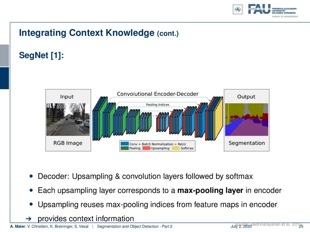
You see integrating context knowledge is key. In SegNet, a different approach was taken here. You also have this encoder-decoder structure that is convolutional. Here, the key idea was that in the upsampling step, you reuse the information from the max-pooling in the downsampling steps such that you get better-resolved decoding. This is already a pretty good idea to integrate the context knowledge.
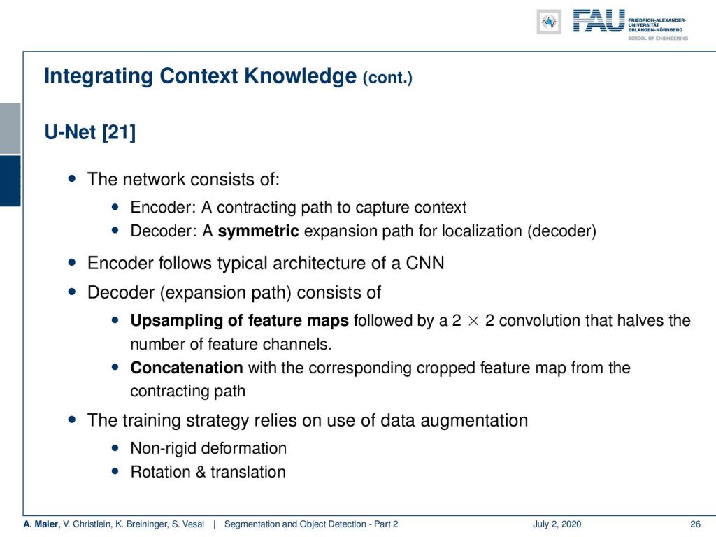
An even better idea is then demonstrated in U-net. Here, the network consists of the encoder branch which is then a contracting path to capture the context. The decoder branch does symmetric expansion for the localization. So, the encoder follows the typical structure of a CNN. The decoder now consists of the upsampling step and a concatenation of the previous feature maps of the respective layers of the corresponding encoder step. So, then the training strategy relies also on data augmentation. There were non-rigid deformations, rotations, and translations that were used to give the U-net an additional kick of performance.
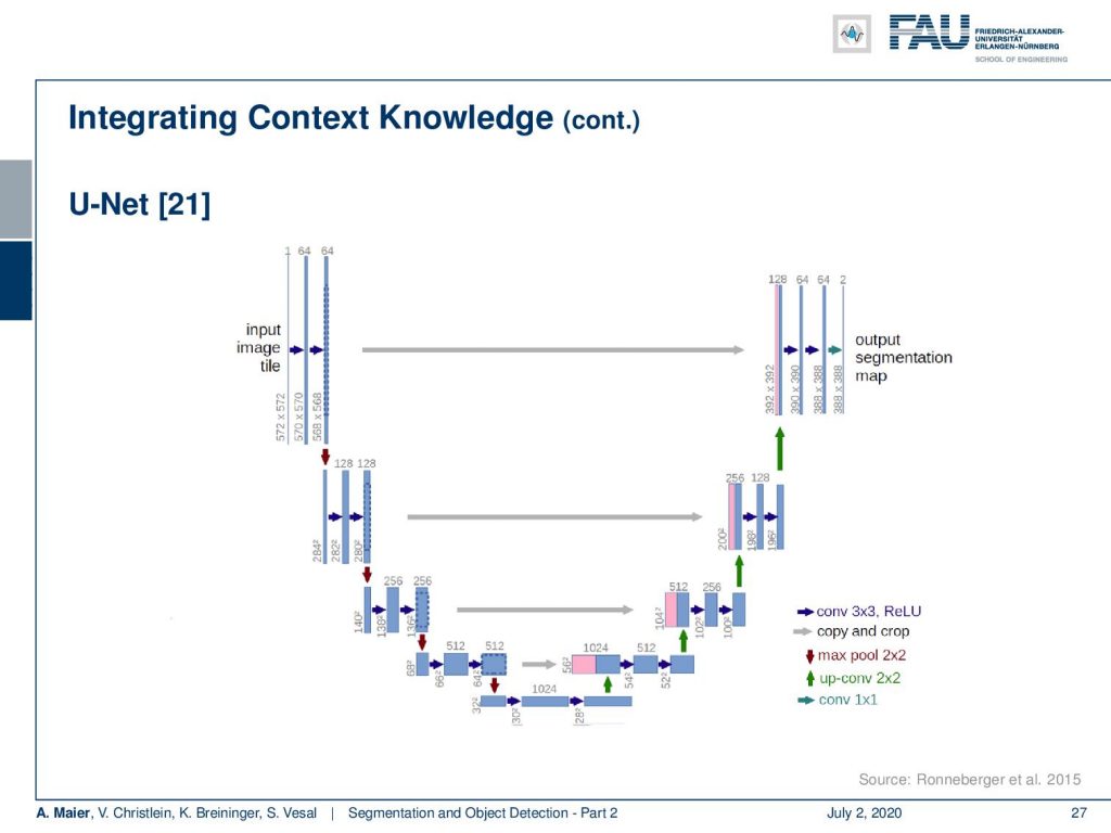
You can say that U-net is essentially the state-of-the-art method for image segmentation. This is also the reason why it has this name. It stems from its shape. You can see that you get this U structure because you have a high resolution on the fine levels. Then you downsample to a lower resolution. The decoder branch upsamples everything again. The key information is here the skip connections that are connecting the two respective levels of the decoder and the encoder. This way you can get very, very good image segmentation. It’s quite straightforward to train and this paper has been cited thousands of times (August 11th, 2020: 16471 citations). Every day you can check the citation count and it already increased. Olaf Ronneberger was able to publish a very important paper here and it’s dominating the entire scene of image segmentation.
You can see that there are many additional approaches. They can be implemented with the U-net. So they can use dilated convolutions and many more. There have been many of these very small changes that have been suggested and they may be useful for particular tasks but for general image segmentation, the U-net has been shown to still outperform such approaches. Still, there are things using like dilated convolutions, there are network stacks that can be very beneficial, and there’s also multi-scale networks that then even further go into this idea of using the image at different scales. You can also do things like deferring the context modeling to another network. Then, you can also incorporate recurrent neural networks. Also very nice is the idea to refine the resulting segmentation maps using a conditional random field.
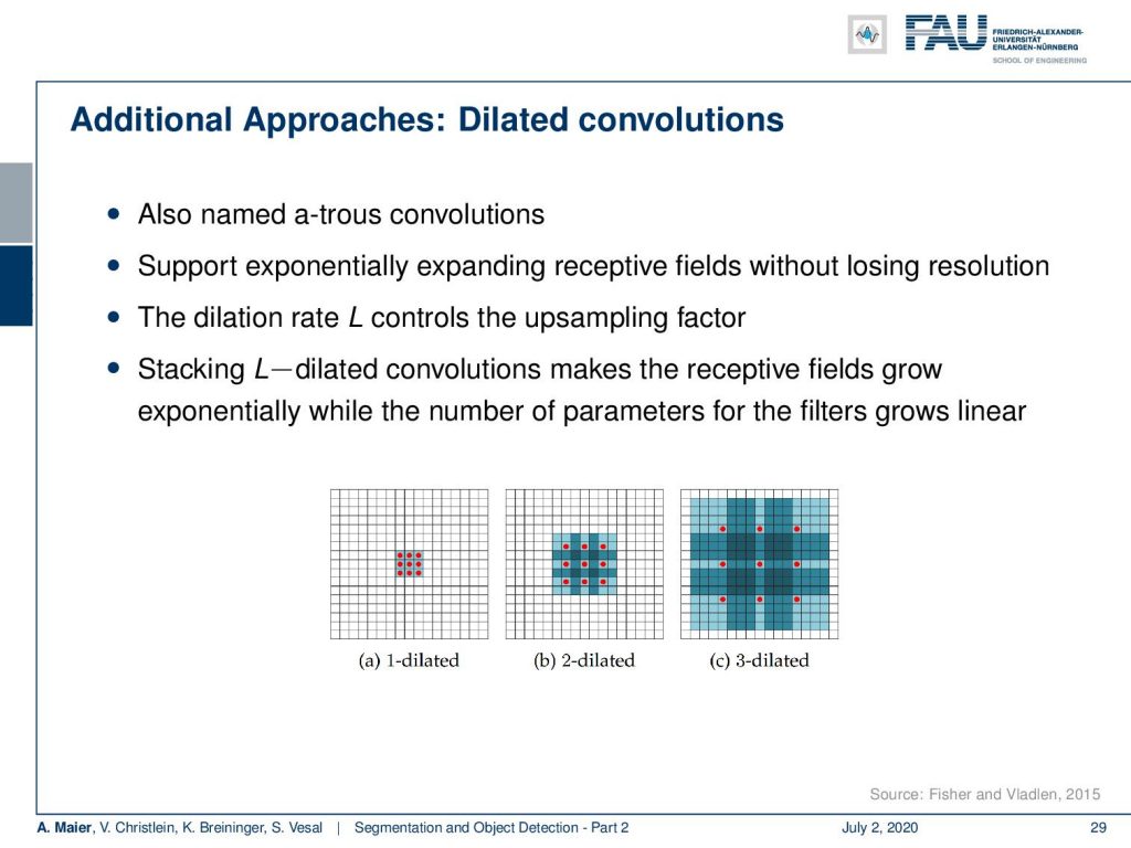
We have some of these additional approaches here, such that you can see what we are talking about. The dilated convolutions, here, is the idea that you want to use those atrous convolutions that we already talked about. So, the idea is that you use dilated convolutions to support exponentially expanding the receptive field without losing the resolution. Then, you introduce the dilation rate L that controls the upsampling factor. You then stack this on top such that you make the receptive field grow exponentially while the number of parameters for the filters grows linear. So, in specific applications where you have a broad range of magnifications happening, this can be very useful. So, it really depends on your application.
Examples for this are DeepLab, ENet, and the multi-scale context aggregation module in [28]. The main issue, of course, is there’s no efficient implementation available. So, the benefit is somewhat unclear.
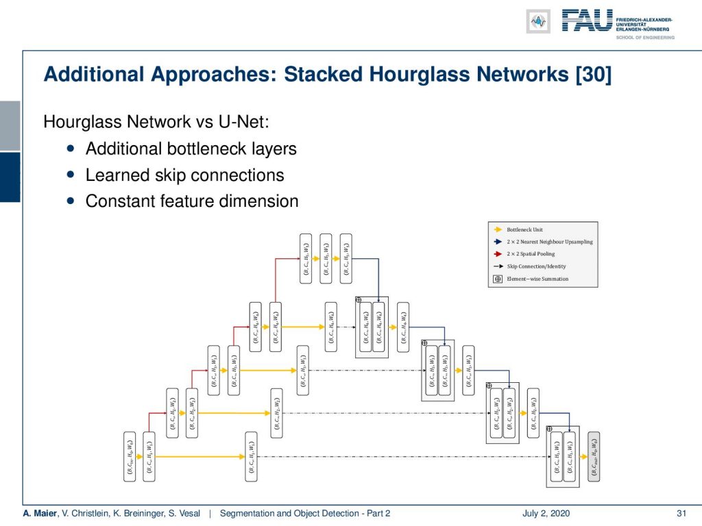
Another approach that I would like to show you here is these so-called stacked hourglass network. So, here, the idea is that you use something very similar to a U-net, but you would put in an additional trainable part in the skip connection. So, that’s essentially the main idea.
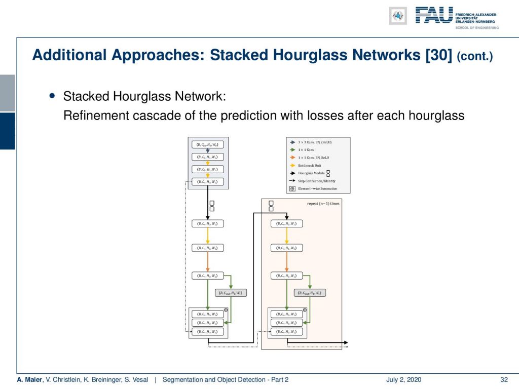
Then, you can use this hourglass module and stack it behind each other. So, you have essentially multiple refinement steps after each other and you always return to the original resolution. You can plug in a second network essentially as a kind of artifact correction network. Now, what’s really nice about this kind of hourglass network approach is that you return to the original resolution.
Let’s say you’re predicting several classes at the same time. Then, you end up with several segmentation masks for the different classes. This idea can then be picked up in something that is called a convolutional pose machine. In the convolutional pose machine, you then use the area where your hourglasses connect, where you have one U-net essentially stacked on top of another U-net. At this layer, you can then also use the resulting segmentation maps per class in order to inform them of each other. So, you can use the context information of other things that have been detected in the image in order to steer this refinement. In convolutional pose machines, you do that for pose detection of joints of a body model. Of course, if you have the left knee joint and the right knee joint and other joints of the body the information about the other joints helps in decoding the correct position.
This idea has also been used by my colleague Bastian Bier for the detection of anatomic landmarks in the analysis of x-ray projections. I’m showing a small video here. You’ve already seen that in the introduction and now you finally have all the context that you need to understand the method. So, here you have an approach behind it that is very similar to convolutional pose machines that then start informing the landmarks about each other’s orientation and position in order to get improved detection results.
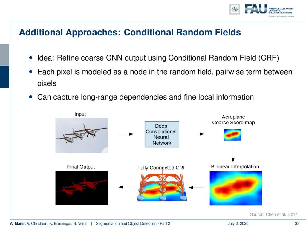
So what else? I already hinted at the conditional random fields. Here, the idea is that you refine the output using a conditional random field. So, the pixel is modeled as a node in a random field. Theses pair-based terms between the pixels are very interesting because they can capture long-range dependencies and fine, local information.
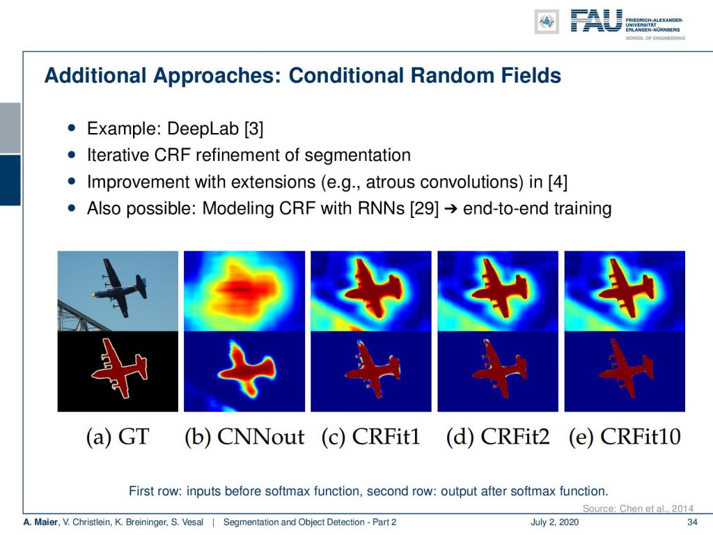
So if you see the output here, this is from DeepLab. Here, you see how the iterative refinement of the conditional random field then can help to improve the segmentation. So, you can then also combine this with artous convolutions as in [4]. You could even model the conditional random field with recurrent neural networks as shown in reference [29]. This then also allows end-to-end training of the entire conditional random field.
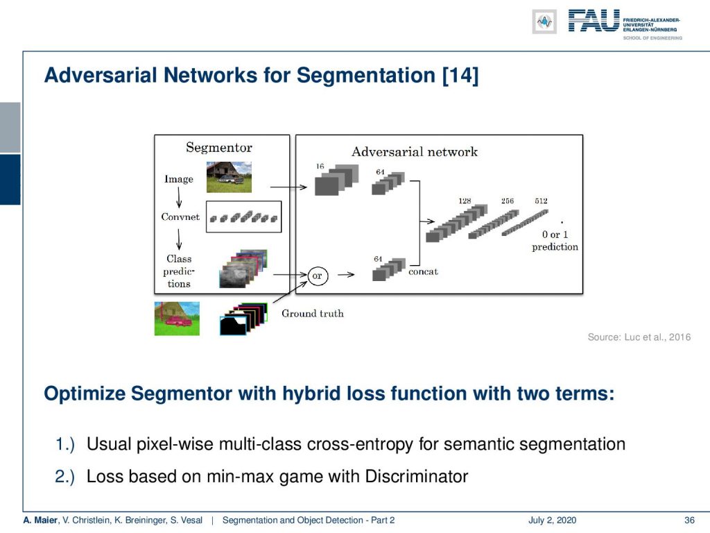
There are also a couple of advanced topics that I still want to hint at. Of course, you can also work with the losses. So far, we’ve only seen the segmentation loss itself but of course, you can also mix and match from previous ideas that we already saw in this class. For example, you can use a GAN in order to augment your loss. The idea here is then that you can essentially create a segmentor. You can then use the output of the segmentor as an input to a GAN type of discriminator. The discriminator now gets the task to say whether this is an automatic segmentation or a manual one. Then, this can be used as a kind of additional adversarial loss inspired by the ideas of the generative adversarial networks. You find that very often in literature as the so-called adversarial loss.
So, how is this then implemented? Well, the idea is that if you have a data set given of N training images and the corresponding label maps, you can then build the following loss function: This is essentially the multi-class cross-entropy loss and then you put on top the adversarial loss that works on your segmentation masks. So here, you can then essentially train your segmentation both with the ground truth label and on fooling the discriminator. This is essentially nothing else than a multi-task learning approach with an adversarial task.
Okay. So, this already brings us to the end of our short video today. You see that we’ve seen now the key ideas on how to build good segmentation networks. In particular, U-net is one of the key ideas that you should know about. Now that we have discussed the segmentation networks, we can talk in the next lecture about object detection and how to actually implement that very quickly. So, this is the other side of image interpretation. We will also be able to figure out where different instances in the image actually are. So I hope, you liked this small video and I’m looking forward to seeing you in the next one. Thank you very much and bye-bye.
If you liked this post, you can find more essays here, more educational material on Machine Learning here, or have a look at our Deep LearningLecture. I would also appreciate a follow on YouTube, Twitter, Facebook, or LinkedIn in case you want to be informed about more essays, videos, and research in the future. This article is released under the Creative Commons 4.0 Attribution License and can be reprinted and modified if referenced. If you are interested in generating transcripts from video lectures try AutoBlog.
References
[1] Vijay Badrinarayanan, Alex Kendall, and Roberto Cipolla. “Segnet: A deep convolutional encoder-decoder architecture for image segmentation”. In: arXiv preprint arXiv:1511.00561 (2015). arXiv: 1311.2524.
[2] Xiao Bian, Ser Nam Lim, and Ning Zhou. “Multiscale fully convolutional network with application to industrial inspection”. In: Applications of Computer Vision (WACV), 2016 IEEE Winter Conference on. IEEE. 2016, pp. 1–8.
[3] Liang-Chieh Chen, George Papandreou, Iasonas Kokkinos, et al. “Semantic Image Segmentation with Deep Convolutional Nets and Fully Connected CRFs”. In: CoRR abs/1412.7062 (2014). arXiv: 1412.7062.
[4] Liang-Chieh Chen, George Papandreou, Iasonas Kokkinos, et al. “Deeplab: Semantic image segmentation with deep convolutional nets, atrous convolution, and fully connected crfs”. In: arXiv preprint arXiv:1606.00915 (2016).
[5] S. Ren, K. He, R. Girshick, et al. “Faster R-CNN: Towards Real-Time Object Detection with Region Proposal Networks”. In: vol. 39. 6. June 2017, pp. 1137–1149.
[6] R. Girshick. “Fast R-CNN”. In: 2015 IEEE International Conference on Computer Vision (ICCV). Dec. 2015, pp. 1440–1448.
[7] Tsung-Yi Lin, Priya Goyal, Ross Girshick, et al. “Focal loss for dense object detection”. In: arXiv preprint arXiv:1708.02002 (2017).
[8] Alberto Garcia-Garcia, Sergio Orts-Escolano, Sergiu Oprea, et al. “A Review on Deep Learning Techniques Applied to Semantic Segmentation”. In: arXiv preprint arXiv:1704.06857 (2017).
[9] Bharath Hariharan, Pablo Arbeláez, Ross Girshick, et al. “Simultaneous detection and segmentation”. In: European Conference on Computer Vision. Springer. 2014, pp. 297–312.
[10] Kaiming He, Georgia Gkioxari, Piotr Dollár, et al. “Mask R-CNN”. In: CoRR abs/1703.06870 (2017). arXiv: 1703.06870.
[11] N. Dalal and B. Triggs. “Histograms of oriented gradients for human detection”. In: 2005 IEEE Computer Society Conference on Computer Vision and Pattern Recognition Vol. 1. June 2005, 886–893 vol. 1.
[12] Jonathan Huang, Vivek Rathod, Chen Sun, et al. “Speed/accuracy trade-offs for modern convolutional object detectors”. In: CoRR abs/1611.10012 (2016). arXiv: 1611.10012.
[13] Jonathan Long, Evan Shelhamer, and Trevor Darrell. “Fully convolutional networks for semantic segmentation”. In: Proceedings of the IEEE Conference on Computer Vision and Pattern Recognition. 2015, pp. 3431–3440.
[14] Pauline Luc, Camille Couprie, Soumith Chintala, et al. “Semantic segmentation using adversarial networks”. In: arXiv preprint arXiv:1611.08408 (2016).
[15] Christian Szegedy, Scott E. Reed, Dumitru Erhan, et al. “Scalable, High-Quality Object Detection”. In: CoRR abs/1412.1441 (2014). arXiv: 1412.1441.
[16] Hyeonwoo Noh, Seunghoon Hong, and Bohyung Han. “Learning deconvolution network for semantic segmentation”. In: Proceedings of the IEEE International Conference on Computer Vision. 2015, pp. 1520–1528.
[17] Adam Paszke, Abhishek Chaurasia, Sangpil Kim, et al. “Enet: A deep neural network architecture for real-time semantic segmentation”. In: arXiv preprint arXiv:1606.02147 (2016).
[18] Pedro O Pinheiro, Ronan Collobert, and Piotr Dollár. “Learning to segment object candidates”. In: Advances in Neural Information Processing Systems. 2015, pp. 1990–1998.
[19] Pedro O Pinheiro, Tsung-Yi Lin, Ronan Collobert, et al. “Learning to refine object segments”. In: European Conference on Computer Vision. Springer. 2016, pp. 75–91.
[20] Ross B. Girshick, Jeff Donahue, Trevor Darrell, et al. “Rich feature hierarchies for accurate object detection and semantic segmentation”. In: CoRR abs/1311.2524 (2013). arXiv: 1311.2524.
[21] Olaf Ronneberger, Philipp Fischer, and Thomas Brox. “U-net: Convolutional networks for biomedical image segmentation”. In: MICCAI. Springer. 2015, pp. 234–241.
[22] Kaiming He, Xiangyu Zhang, Shaoqing Ren, et al. “Spatial Pyramid Pooling in Deep Convolutional Networks for Visual Recognition”. In: Computer Vision – ECCV 2014. Cham: Springer International Publishing, 2014, pp. 346–361.
[23] J. R. R. Uijlings, K. E. A. van de Sande, T. Gevers, et al. “Selective Search for Object Recognition”. In: International Journal of Computer Vision 104.2 (Sept. 2013), pp. 154–171.
[24] Wei Liu, Dragomir Anguelov, Dumitru Erhan, et al. “SSD: Single Shot MultiBox Detector”. In: Computer Vision – ECCV 2016. Cham: Springer International Publishing, 2016, pp. 21–37.
[25] P. Viola and M. Jones. “Rapid object detection using a boosted cascade of simple features”. In: Proceedings of the 2001 IEEE Computer Society Conference on Computer Vision Vol. 1. 2001, pp. 511–518.
[26] J. Redmon, S. Divvala, R. Girshick, et al. “You Only Look Once: Unified, Real-Time Object Detection”. In: 2016 IEEE Conference on Computer Vision and Pattern Recognition (CVPR). June 2016, pp. 779–788.
[27] Joseph Redmon and Ali Farhadi. “YOLO9000: Better, Faster, Stronger”. In: CoRR abs/1612.08242 (2016). arXiv: 1612.08242.
[28] Fisher Yu and Vladlen Koltun. “Multi-scale context aggregation by dilated convolutions”. In: arXiv preprint arXiv:1511.07122 (2015).
[29] Shuai Zheng, Sadeep Jayasumana, Bernardino Romera-Paredes, et al. “Conditional Random Fields as Recurrent Neural Networks”. In: CoRR abs/1502.03240 (2015). arXiv: 1502.03240.
[30] Alejandro Newell, Kaiyu Yang, and Jia Deng. “Stacked hourglass networks for human pose estimation”. In: European conference on computer vision. Springer. 2016, pp. 483–499.