
Normalization & Dropout
These are the lecture notes for FAU’s YouTube Lecture “Deep Learning“. This is a full transcript of the lecture video & matching slides. We hope, you enjoy this as much as the videos. Of course, this transcript was created with deep learning techniques largely automatically and only minor manual modifications were performed. If you spot mistakes, please let us know!
Welcome to our deep learning lecture. Today we want to talk about a bit more regularization. The first topic that I want to introduce is an idea of normalization. So why could normalization be a problem?
Let’s look at some original data here. A typical approach is that you subtract the mean and then you can also normalize the variance. This is very useful because then we’re in an expected range regarding the input. Of course, if you do these normalizations, then you want to estimate them only on the training data. Another approach is not just to normalize before the network but you can also normalize within the network. This then leads to the concept of batch normalization.
The idea is to introduce a new layer with parameters γ and β. γ and β are being used to rescale the output of the layer. At the input of the layer, you start measuring the mean and the standard deviation of the batch. So what you do is you compute over the mini-batch, the current mean and standard deviation, and then you use that to normalize the activations of the input. As a result, you have a zero mean and unit standard deviation. So this is calculated on the fly throughout the training process and then you scale at the output of the layer with the trainable weights β and γ. You scale them appropriately as desired for the next layer. So this nice feature can of course only be done during the training. If you want to move on towards test time, you compute – after you finish the training – the mean and the standard deviation in the batch normalization layer once for the entire training set and you keep it and constant for all future applications of the network. Of course, μ and σ are vectors and they have exactly the same dimension as the activation vector. Typically, you pair this with convolutional layers. In this case, the batch normalization is slightly different by using a scalar μ and a σ for every channel. So there’s a slight difference if you use it in convolution.
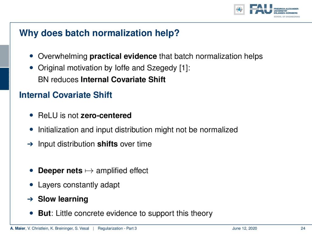
You may argue why does batch normalization actually help? There’s overwhelming practical evidence that it’s really a useful tool and this has been originally motivated by the internal covariate shift. So, the problem that the ReLU is not zero centered was identified. Hence, initialization and input distribution may not be normalized. Therefore, the input distribution shifts over time. In deeper nets, you even get an amplified effect. As a result, the layers constantly have to adapt and this leads to slow learning. Now, if you look at these observations closely, there is very little concrete evidence to support this theory.
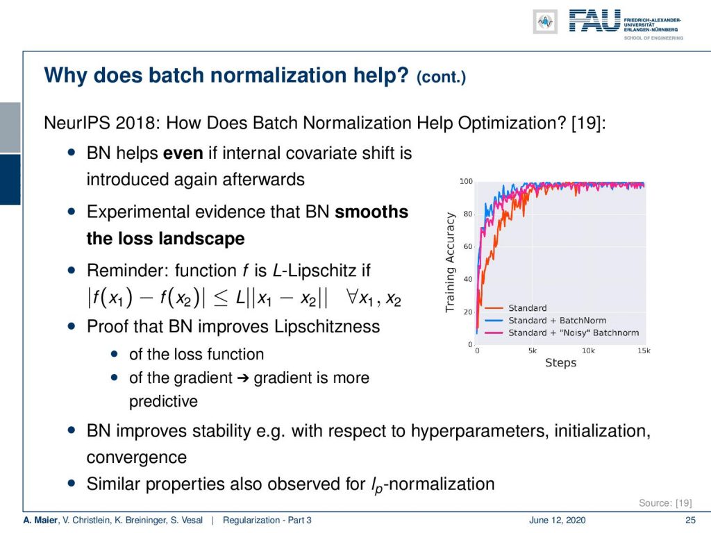
On NeurIPS 2018, there was a paper that showed how batch normalization helps optimization. They showed that batch normalization is effective even if you introduce an internal covariate shift after the batch normalization layer again. So still in these situations batch normalization helped. They could show experimentally that the method smoothes the loss landscape. This supports the optimization and also helped to lower the Lipschitzness of the loss function. The Lipschitz constant is the highest slope that occurs in the function. If you improve the Lipchitzness it essentially means that high slopes do no longer occur. So this is in line with smoothing the loss landscape. They even could provide proof for this property in the paper. So batch normalization improves stability with respect to hyperparameters, initialization, convergence, and similar properties. By the way, this can also be observed for Lp normalization.
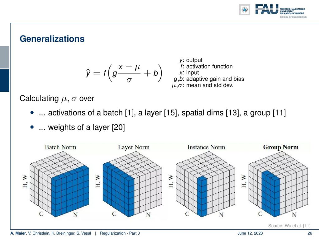
So that’s one way to go. There are generalizations of batch normalization: You can calculate the μ and the σ over activations of a batch, over a layer, over spatial dimensions, over a group, over the weights of layer, and we might have missed some variations. So it is a very powerful tool.
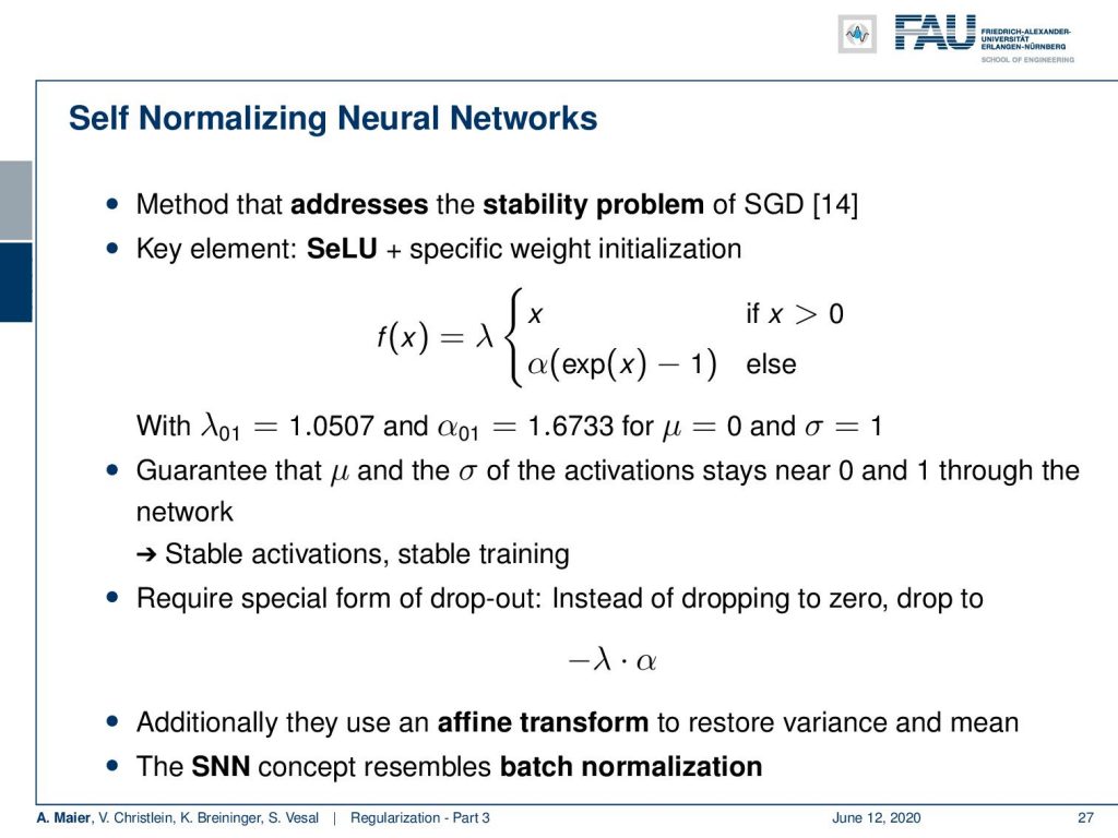
Another tool that is also very effective is the self normalizing neural network. It also addresses the stability problem of stochastic gradient descent and the key element here is the scaled exponential linear unit that we already discussed in the activation functions. So, here we have the definition again. With the particular setting for λ and for α, we can ensure the property that a zero mean and unit standard deviation input will have the same mean and standard deviation at the output of the data. So this is guaranteed to keep these properties. Then the result is that stable activations also lead to stable training. One thing that has to be changed is the dropout procedure which we will look at in the next paragraph. Here instead of dropping to zero, you have to drop to minus λ times α. Additionally, they use an affine transform to restore the variance and the mean. So this self normalizing neural network concept to some extent also resembles the batch normalization. Interestingly, it also leads to increased stability and it’s also a good recipe that you may want to consider when building your neural networks.
Now we already talked about dropout. It is also a very important technology that is being used in deep networks. One thing that you may want to consider is that all of the elements during training, of course, they depend on each other. So, if you have correlated inputs then also the adaptation will run in a similar way. But if you want to have independent features that allow you to recognize different things, then you somehow have to break the correlation between the features and this can actually be performed by dropout. It is essentially the idea that you randomly kill some of the neurons and just set them to zero. So you select a probability p and you set random activations to zero with probability 1 – p. Then during test time of course you have to multiply all of the activations with p because otherwise, you would have a too high activation in the next layer. So you have to compensate for this dropout effect at the test time. Let’s say y₁ and y₂ in this example, they would be correlated so they carried the same information and weights. Now, if I use them and try to train them, they will never learn something else because they always produce the same output. Thus, in the backpropagation, they will get the same update term. Hence, they will always stay correlated. Now if you introduce this dropout procedure, you randomly kill some of the neurons. This means that during the training procedure, the weights get drawn in a different direction. Therefore, they will no longer be correlated. So, you can break these internal correlations using dropout and this has shown to reduce problems of overfitting. This is really a very important concept that quite frequently is used in deep learning. Also interesting is a generalization that is dropconnect. Here, you don’t kill all of the activations of an individual neuron, but you kill the individual connections. So you randomly identify connections that are set to zero. This could be seen as a generalization of dropout because do you have more different ways of adjusting it. Typically, the implementation is not as efficient because you have to implement this as masking. It’s simpler just to set one of the activations to zero.
Okay so we already talked about these common concepts and normalization but that’s not all tricks of the trade. We still have a couple of cards up in our sleeves. So these tricks I will show you in the next lecture. Thank you very much for listening and goodbye!
If you liked this post, you can find more essays here, more educational material on Machine Learning here, or have a look at our Deep LearningLecture. I would also appreciate a clap or a follow on YouTube, Twitter, Facebook, or LinkedIn in case you want to be informed about more essays, videos, and research in the future. This article is released under the Creative Commons 4.0 Attribution License and can be reprinted and modified if referenced.
Links
Link – for details on Maximum A Posteriori estimation and the bias-variance decomposition
Link – for a comprehensive text about practical recommendations for regularization
Link – the paper about calibrating the variances
References
[1] Sergey Ioffe and Christian Szegedy. “Batch Normalization: Accelerating Deep Network Training by Reducing Internal Covariate Shift”. In: Proceedings of The 32nd International Conference on Machine Learning. 2015, pp. 448–456.
[2] Jonathan Baxter. “A Bayesian/Information Theoretic Model of Learning to Learn via Multiple Task Sampling”. In: Machine Learning 28.1 (July 1997), pp. 7–39.
[3] Christopher M. Bishop. Pattern Recognition and Machine Learning (Information Science and Statistics). Secaucus, NJ, USA: Springer-Verlag New York, Inc., 2006.
[4] Richard Caruana. “Multitask Learning: A Knowledge-Based Source of Inductive Bias”. In: Proceedings of the Tenth International Conference on Machine Learning. Morgan Kaufmann, 1993, pp. 41–48.
[5] Andre Esteva, Brett Kuprel, Roberto A Novoa, et al. “Dermatologist-level classification of skin cancer with deep neural networks”. In: Nature 542.7639 (2017), pp. 115–118.
[6] C. Ding, C. Xu, and D. Tao. “Multi-Task Pose-Invariant Face Recognition”. In: IEEE Transactions on Image Processing 24.3 (Mar. 2015), pp. 980–993.
[7] Li Wan, Matthew Zeiler, Sixin Zhang, et al. “Regularization of neural networks using drop connect”. In: Proceedings of the 30th International Conference on Machine Learning (ICML-2013), pp. 1058–1066.
[8] Nitish Srivastava, Geoffrey E Hinton, Alex Krizhevsky, et al. “Dropout: a simple way to prevent neural networks from overfitting.” In: Journal of Machine Learning Research 15.1 (2014), pp. 1929–1958.
[9] R. O. Duda, P. E. Hart, and D. G. Stork. Pattern Classification. John Wiley and Sons, inc., 2000.
[10] Ian Goodfellow, Yoshua Bengio, and Aaron Courville. Deep Learning. http://www.deeplearningbook.org. MIT Press, 2016.
[11] Yuxin Wu and Kaiming He. “Group normalization”. In: arXiv preprint arXiv:1803.08494 (2018).
[12] Kaiming He, Xiangyu Zhang, Shaoqing Ren, et al. “Delving deep into rectifiers: Surpassing human-level performance on imagenet classification”. In: Proceedings of the IEEE international conference on computer vision. 2015, pp. 1026–1034.
[13] D Ulyanov, A Vedaldi, and VS Lempitsky. Instance normalization: the missing ingredient for fast stylization. CoRR abs/1607.0 [14] Günter Klambauer, Thomas Unterthiner, Andreas Mayr, et al. “Self-Normalizing Neural Networks”. In: Advances in Neural Information Processing Systems (NIPS). Vol. abs/1706.02515. 2017. arXiv: 1706.02515.
[15] Jimmy Lei Ba, Jamie Ryan Kiros, and Geoffrey E Hinton. “Layer normalization”. In: arXiv preprint arXiv:1607.06450 (2016).
[16] Nima Tajbakhsh, Jae Y Shin, Suryakanth R Gurudu, et al. “Convolutional neural networks for medical image analysis: Full training or fine tuning?” In: IEEE transactions on medical imaging 35.5 (2016), pp. 1299–1312.
[17] Yoshua Bengio. “Practical recommendations for gradient-based training of deep architectures”. In: Neural networks: Tricks of the trade. Springer, 2012, pp. 437–478.
[18] Chiyuan Zhang, Samy Bengio, Moritz Hardt, et al. “Understanding deep learning requires rethinking generalization”. In: arXiv preprint arXiv:1611.03530 (2016).
[19] Shibani Santurkar, Dimitris Tsipras, Andrew Ilyas, et al. “How Does Batch Normalization Help Optimization?” In: arXiv e-prints, arXiv:1805.11604 (May 2018), arXiv:1805.11604. arXiv: 1805.11604 [stat.ML].
[20] Tim Salimans and Diederik P Kingma. “Weight Normalization: A Simple Reparameterization to Accelerate Training of Deep Neural Networks”. In: Advances in Neural Information Processing Systems 29. Curran Associates, Inc., 2016, pp. 901–909.
[21] Xavier Glorot and Yoshua Bengio. “Understanding the difficulty of training deep feedforward neural networks”. In: Proceedings of the Thirteenth International Conference on Artificial Intelligence 2010, pp. 249–256.
[22] Zhanpeng Zhang, Ping Luo, Chen Change Loy, et al. “Facial Landmark Detection by Deep Multi-task Learning”. In: Computer Vision – ECCV 2014: 13th European Conference, Zurich, Switzerland, Cham: Springer International Publishing, 2014, pp. 94–108.