Lecture Notes in Deep Learning: Regularization – Part 2

Classical Techniques

These are the lecture notes for FAU’s YouTube Lecture “Deep Learning“. This is a full transcript of the lecture video & matching slides. We hope, you enjoy this as much as the videos. Of course, this transcript was created with deep learning techniques largely automatically and only minor manual modifications were performed. If you spot mistakes, please let us know!

Welcome back to Deep Learning! We want to continue our analysis of regularization methods and today I want to talk about classical techniques.

So here is a typical example of a loss curve over the iterations on the training set. What I show here on the right-hand side is the loss curve on the test set. You see that although the training loss goes down the test loss goes up. So at some point, the training data set is overfitted and it doesn’t produce a model that is representative of the data anymore. By the way, always keep in mind that the test set must never be used for training. If you’re trained on your test set, then you will get very good results but it’s very likely to be a complete overestimate of the performance. So there’s the typical situation that somebody who runs into my office and says: “Yes! I have 99% recognition rate!”. The first thing that somebody in pattern recognition or machine learning does when he reads “99% recognition rate” is ask: “Did you train on your test data?” This is the very first thing you make sure that has not happened. When you did some stupid mistake, there’s some data set pointer that was not pointing to the right data set and suddenly your recognition rate jumps up. So, be careful if you have very good results. Always scrutinize that they are really appropriate and they’re really general. So instead if you want to produce curves like the ones that I’m showing here you may want to use a validation set that you take off the training data set. You never use this set in training but you can use it to get an estimate for your model overfitting.

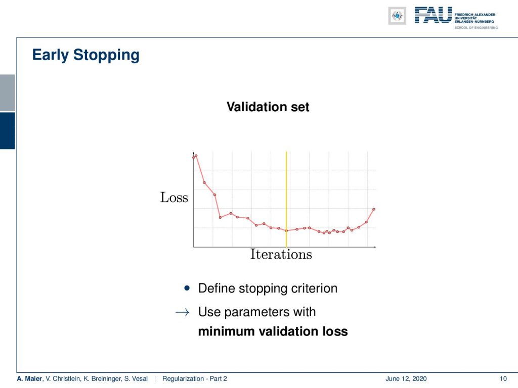
So, if you do that then we can already use the first trick. You use the validation set. We observe at what point we have the minimum error in the validation set is. If we’re at this point, we can use that as a stopping criterion and use that model for our test evaluation. So it’s a common technique to use the parameters with the minimum validation results.

Another very useful technique is data augmentation. So, the idea here is to artificially enlarge the data set. There are transformations on the label which should be invariant to the class. Let’s say you have the image of a cat and you rotate it by 90 degrees, it still shows a cat. Obviously, those augmentation techniques have to be done carefully. So, in the right-hand example, you can see that a rotation by 180 degrees is probably not a good way of augmenting numbers, because it may switch the label.

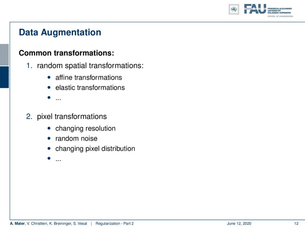
So, there are very common transformations here: Random spatial transforms like affine or elastic transforms. Then, there are pixel transforms like changing the resolution, changing noise, or changing pixel distributions like color brightness, and so on. So these are typical augmentation techniques in image processing.

What else? We can regularize the loss function. Here, we can see that this essentially leads to the maximum a-posteriori (MAP) estimation. We can do this in a Bayesian approach where we want to consider the uncertain weights w. They follow a prior distribution p(w). If you have some data set X with some associated labels Y, we can see that the joint probability p(w, Y, X) is the probability p(w|Y, X) times the probability p(Y, X). We can reformulate that into the probability P(Y|X, w) times the probability p(X, w). From these equalities, we can derive the Bayes theorem that the conditional probability p(w|Y, X) can be expressed as the probability p(Y|X, w) times the probability P(X, w) divided by the probability p(Y, X). So this, we can rearrange a bit further and here you see that then the probability p(X) the probability p(Y|X) pop up. By removing the terms that are independent of w, this yields the MAP estimate. So, we can actually seek to maximize the joint probability as maximizing the conditional probability p(Y|X, w) times the probability p(w). So typically, we solve this as a maximum likelihood estimator following the left-hand side problem times the prior on w which is the right-hand side part. We can say this is a maximum likelihood estimator, but we augment it with some additional prior information. Here, the prior information is that we have some knowledge about the distribution of w for example w could be sparse. We can also use some other source of knowledge where we know something about w. In image processing what is used very often is for example that natural images are sparse with respect to the gradients so there are all kinds of sparsities that can be employed by such a prior.

Now the interesting part is that this MAP estimator can be reformulated and if you attended pattern recognition, you know what I’m talking about. We’ve seen that the maximization of the maximum likelihood estimates results in a minimization of the negative log-likelihood. The typical loss functions that we’re talking about have this form. Now, if you start with the map estimate, you essentially end up with a very similar estimate but the shape of the loss function has slightly changed. So, we get a new loss function L tilde. It’s like the L2 loss or the cross-entropy loss plus some λ and some constraint on the weights w. So here, we enforce a minimum l2 norm. Now with a positive λ, we can identify this by the way as the lagrangian function of minimizing the loss function subject to constrained L2 norm of w being smaller than α with some unknown data-dependent α. So this is exactly the same formulation. We can now bring this into the backpropagation of the augmented loss. How this is typically implemented? You follow the loss of the gradient. So, this is the right-hand part of the loss that we already computed with the learning rate η and in addition, you apply this kind of shrinkage to w. So, the shrinkage step here can be used in order to implement the additional L2 regularization. So the nice thing is now that we can simply compute the backpropagation as we used to do it. Then, in addition, we use the shrinkage in the weight update. So we also get very simple weight updates and they allow us to involve those regularizers. If we choose different regularizers, the shrinkage functions change. If we would optimize the training loss now for λ we would usually receive λ = 0 because every time we introduce regularization, we are doing something that is not optimal with respect to training loss. Of course, we introduced it because we want to reduce overfitting. So this is something that we cannot observe directly in our training data but we want to get better properties on an unseen test set. This will even increase the loss value of our training data. So be careful of that. Again, we increase the bias for a reduced variance.

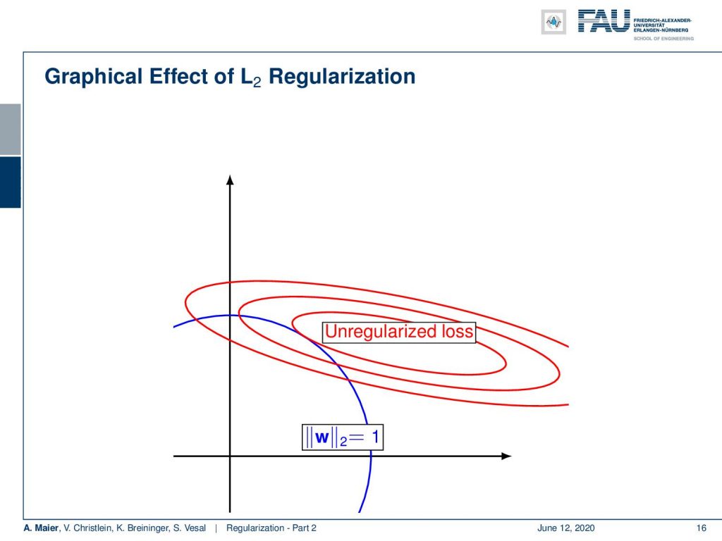
Here, we have a visualization of the effect of the L2 regularizer. The unregularized loss would of course result in the center of the ellipses in red. But now you do the additional regularization which enforces your w to be small. This means that the farther you away from the origin the higher your L2 loss will be. So, the l2 loss pulls you away from the data optimal loss with respect to your training dataset. Hopefully, it describes some prior knowledge that we haven’t seen this way in the training dataset. Hence, it will then result in a model that is simply better suited for the unseen test data set.

We can also use other norms, for example, the L1 norm. So here, we then again end up in a Lagrangian formulation where we have the original loss function subject to the L1 norm being smaller than some value α with an unknown data-dependent α. Here, we simply get a different shrinkage operation which now involves the use of the sign function. So this is again an implication of the sub-gradient. Here, a different way of shrinkage has to be employed in order to make this optimization feasible. Again, we used exactly the same gradient for loss function as we used previously. So only the shrinkage is replaced.

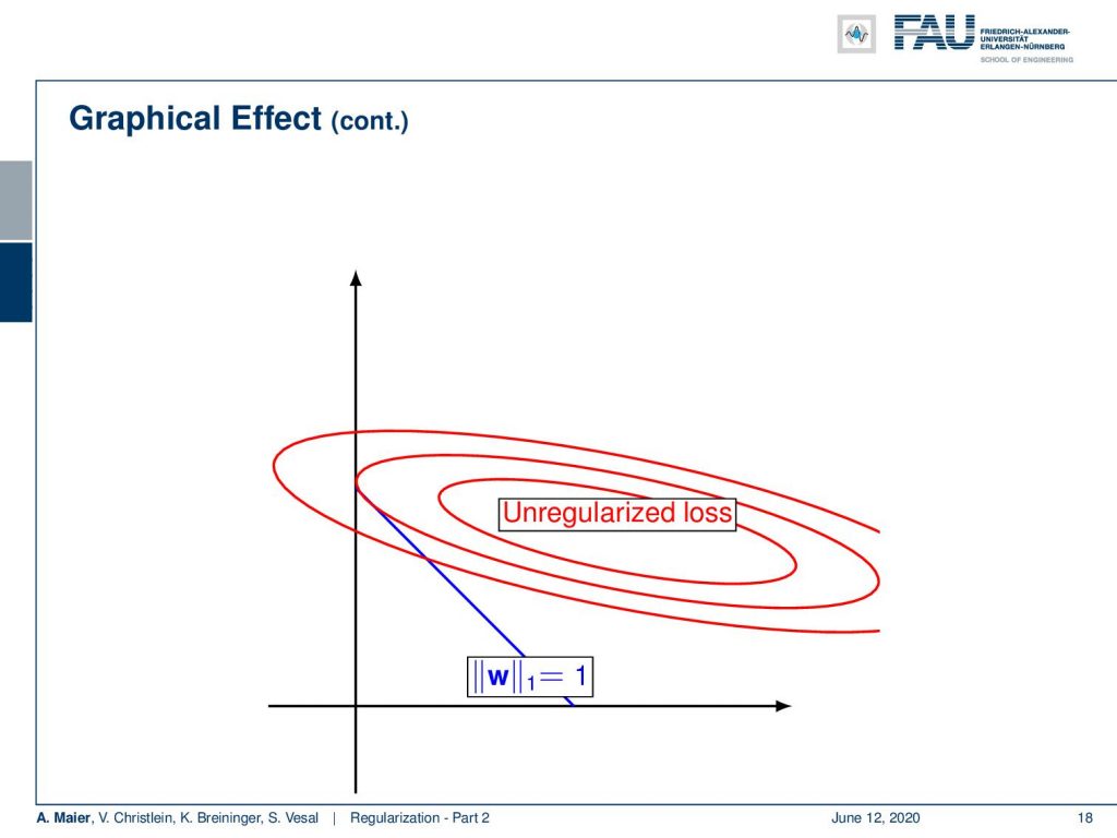
Now, we can also visualize this in our small graph. The shape of the L1 norm is of course different. With L2, we had this circle and with the L1 norm, we get a diamond looking shape. Now, you can see that the minima that are selected are likely to be located on the coordinate axis. So, if you try to find the minimum position of this L1 norm and the unregularized loss, you will see that the point of minimum unregularized loss intersected with this L1 loss is essentially on the y-axis in this plot. This is a solution that is very sparse meaning that we only have entries for y in our weight vector and the entry for x is very close to 0 or equals to 0 in this case. So if you want weights to be sparse or if you want to create networks with few connections, you may want to introduce an additional L1 regularization on the weights. This will cause sparse weights.

What else? There are also more known constraints for example we can set a limit on the norm of the weights. Here, we just enforce them to be below a certain maximum. We want to have the magnitude of w to be below α where α is a positive constant. If you do so, we essentially have to project onto the unit ball with every parameter update and this is again a kind of shrinkage that essentially prohibits exploding gradients. Be careful, it may also simply hide them such that you don’t see them anymore.

There are many other variants of changing the loss. You can have a constraint and an individual λ for every layer. So you could constrain every layer differently but we haven’t seen any gains reported in the literature. Instead of the weights, also the activations can be constrained. This leads to different variants for example in sparse auto-encoders. We will talk about this how they were not regularizing the weights, but the activations to form a specific distribution to produce sparse activations. This is also a very interesting problem and we will talk about this a bit more when we talk about autoencoders and unsupervised learning.

So next time in deep learning, we want to continue to talk about regularization methods. We will look into the very typical ones that are particularly made for deep learning. So very interesting approaches that are slightly different from what you’ve seen in this lecture. So thank you very much for watching and goodbye!

If you liked this post, you can find more essays here, more educational material on Machine Learning here, or have a look at our Deep LearningLecture. I would also appreciate a clap or a follow on YouTube, Twitter, Facebook, or LinkedIn in case you want to be informed about more essays, videos, and research in the future. This article is released under the Creative Commons 4.0 Attribution License and can be reprinted and modified if referenced.

Links

Link – for details on Maximum A Posteriori estimation and the bias-variance decomposition
Link – for a comprehensive text about practical recommendations for regularization
Link – the paper about calibrating the variances

References

[1] Sergey Ioffe and Christian Szegedy. “Batch Normalization: Accelerating Deep Network Training by Reducing Internal Covariate Shift”. In: Proceedings of The 32nd International Conference on Machine Learning. 2015, pp. 448–456.
[2] Jonathan Baxter. “A Bayesian/Information Theoretic Model of Learning to Learn via Multiple Task Sampling”. In: Machine Learning 28.1 (July 1997), pp. 7–39.
[3] Christopher M. Bishop. Pattern Recognition and Machine Learning (Information Science and Statistics). Secaucus, NJ, USA: Springer-Verlag New York, Inc., 2006.
[4] Richard Caruana. “Multitask Learning: A Knowledge-Based Source of Inductive Bias”. In: Proceedings of the Tenth International Conference on Machine Learning. Morgan Kaufmann, 1993, pp. 41–48.
[5] Andre Esteva, Brett Kuprel, Roberto A Novoa, et al. “Dermatologist-level classification of skin cancer with deep neural networks”. In: Nature 542.7639 (2017), pp. 115–118.
[6] C. Ding, C. Xu, and D. Tao. “Multi-Task Pose-Invariant Face Recognition”. In: IEEE Transactions on Image Processing 24.3 (Mar. 2015), pp. 980–993.
[7] Li Wan, Matthew Zeiler, Sixin Zhang, et al. “Regularization of neural networks using drop connect”. In: Proceedings of the 30th International Conference on Machine Learning (ICML-2013), pp. 1058–1066.
[8] Nitish Srivastava, Geoffrey E Hinton, Alex Krizhevsky, et al. “Dropout: a simple way to prevent neural networks from overfitting.” In: Journal of Machine Learning Research 15.1 (2014), pp. 1929–1958.
[9] R. O. Duda, P. E. Hart, and D. G. Stork. Pattern Classification. John Wiley and Sons, inc., 2000.
[10] Ian Goodfellow, Yoshua Bengio, and Aaron Courville. Deep Learning. http://www.deeplearningbook.org. MIT Press, 2016.
[11] Yuxin Wu and Kaiming He. “Group normalization”. In: arXiv preprint arXiv:1803.08494 (2018).
[12] Kaiming He, Xiangyu Zhang, Shaoqing Ren, et al. “Delving deep into rectifiers: Surpassing human-level performance on imagenet classification”. In: Proceedings of the IEEE international conference on computer vision. 2015, pp. 1026–1034.
[13] D Ulyanov, A Vedaldi, and VS Lempitsky. Instance normalization: the missing ingredient for fast stylization. CoRR abs/1607.0 [14] Günter Klambauer, Thomas Unterthiner, Andreas Mayr, et al. “Self-Normalizing Neural Networks”. In: Advances in Neural Information Processing Systems (NIPS). Vol. abs/1706.02515. 2017. arXiv: 1706.02515.
[15] Jimmy Lei Ba, Jamie Ryan Kiros, and Geoffrey E Hinton. “Layer normalization”. In: arXiv preprint arXiv:1607.06450 (2016).
[16] Nima Tajbakhsh, Jae Y Shin, Suryakanth R Gurudu, et al. “Convolutional neural networks for medical image analysis: Full training or fine tuning?” In: IEEE transactions on medical imaging 35.5 (2016), pp. 1299–1312.
[17] Yoshua Bengio. “Practical recommendations for gradient-based training of deep architectures”. In: Neural networks: Tricks of the trade. Springer, 2012, pp. 437–478.
[18] Chiyuan Zhang, Samy Bengio, Moritz Hardt, et al. “Understanding deep learning requires rethinking generalization”. In: arXiv preprint arXiv:1611.03530 (2016).
[19] Shibani Santurkar, Dimitris Tsipras, Andrew Ilyas, et al. “How Does Batch Normalization Help Optimization?” In: arXiv e-prints, arXiv:1805.11604 (May 2018), arXiv:1805.11604. arXiv: 1805.11604 [stat.ML].
[20] Tim Salimans and Diederik P Kingma. “Weight Normalization: A Simple Reparameterization to Accelerate Training of Deep Neural Networks”. In: Advances in Neural Information Processing Systems 29. Curran Associates, Inc., 2016, pp. 901–909.
[21] Xavier Glorot and Yoshua Bengio. “Understanding the difficulty of training deep feedforward neural networks”. In: Proceedings of the Thirteenth International Conference on Artificial Intelligence 2010, pp. 249–256.
[22] Zhanpeng Zhang, Ping Luo, Chen Change Loy, et al. “Facial Landmark Detection by Deep Multi-task Learning”. In: Computer Vision – ECCV 2014: 13th European Conference, Zurich, Switzerland, Cham: Springer International Publishing, 2014, pp. 94–108.

Category: Lecture Notes in Deep Learning