
Bias-Variance Trade-off
These are the lecture notes for FAU’s YouTube Lecture “Deep Learning“. This is a full transcript of the lecture video & matching slides. We hope, you enjoy this as much as the videos. Of course, this transcript was created with deep learning techniques largely automatically and only minor manual modifications were performed. If you spot mistakes, please let us know!
Welcome back to deep learning! So today, we want to talk about regularization techniques and we start with a short introduction to regularization and the general problems of overfitting. So, we will first start about the background. Ask the question “What is the problem of regularization?” Then, we talk about classical techniques, normalization, dropout, initialization, transfer learning, and multitask learning. So why are we talking about this topic so much?
Well, if you want to fit your data then problems like this one would be easy to fit as they have a clear solution. Typically, you have the problem that your data is noisy and you cannot easily separate the classes. So, what you then run into is the problem of underfitting if you have a model that doesn’t have a very high capacity. Then you may have something like this line here which is not a very good fit to describe the separation of the classes. The contrary is overfitting. So here, we have models with very high capacity which try to model everything that they observe in the training data. This may yield decision boundaries that are not very reasonable. What we are actually interested in is a sensible boundary that is somehow a compromise between the observed data and their actual distribution.
So, we can analyze this problem by the so-called bias-variance decomposition. Here, we stick to regression problems where we have an ideal function h(x) that computes some value and it’s typically associated with some measurement noise. So, there’s some additional value ϵ that is added to h(x). It may be distributed normally with a zero mean and a standard deviation of sigma. Now, you can go ahead and use a model to estimate h. This is denoted as f hat that is estimated from some data set D. We can now express the loss for a single point as the expected value of the loss. This would then simply be the L2 loss. So, we take the true function minus the estimated function to the power of two and compute the expected value. Interestingly, this loss can be shown to be decomposable into two parts: There is the bias which is essentially the deviation of the expected value of our model from the true model. So, this essentially measures how far we are off the ground truth. The other part can be explained by the limited size of the data set. We can always try to find a model that is very flexible and tries to reduce bias. What we get as a result is an increase in variance. So, the variance is the expected value of y hat – the current value of y hat to the power of 2. This is nothing else than the variance that we encounter in y hat. Then, of course, there is a small irreproducible error. Now, we can integrate this over every data point in x and we get the loss for the entire data set. By the way, a similar decomposition exists for classification using the 1-0 loss which you can see in [9]. It’s slightly different but it has similar implications. So, we learn that with an increase in variance, we can essentially reduce the bias, i.e. the prediction error of our model on the training dataset.
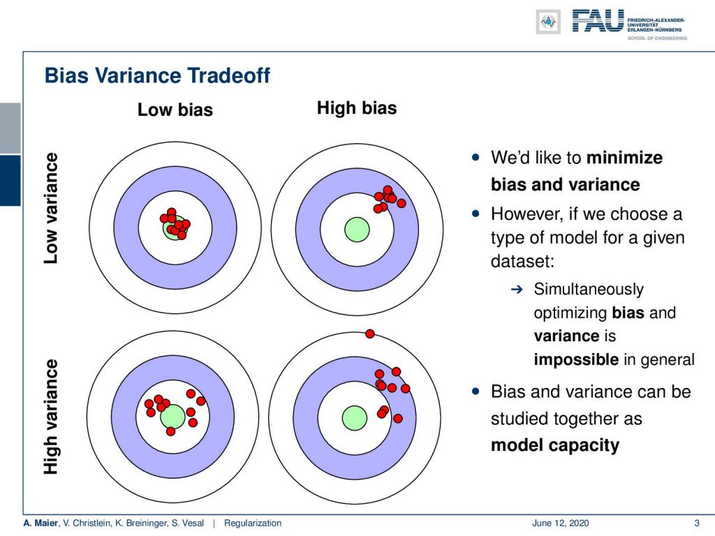
Let’s visualize this a bit: On the top left, we see a low bias, low variance model. This is essentially always right and doesn’t have a lot of noise in the predictions. In the top right, we see a high bias model that is very consistent, i.e. has a low variance and is consistently off. In the bottom left, we see a low bias high, variance model. This has a considerable degree of variation, but on average it’s very close to where it’s supposed to be. In the bottom right, we have the case that we want to omit. This is a high bias, high variance model which has a lot of noise and it’s not even where it’s supposed to be. So, we can choose a type of model for a given data set but simultaneously optimizing bias and variance is in general impossible. Bias and variance can be studied together as model capacity which we’ll look at on the next slide.
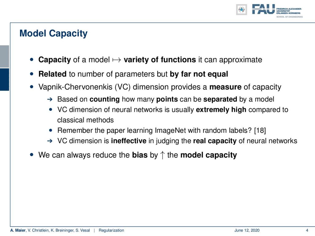
The capacity of a model describes the variety of functions it can approximate. This is related to the number of parameters, so often people say: “That’s the number of parameters. Increase the number of parameters then you can get rid of your bias.” This is true, but it’s by far not equal. To be exact, you need to compute the Vapnik-Chervonenkis (VC) dimension. This is an exact measure of capacity and it’s based on counting how many points can be separated by the model. So, the VC dimension of neural networks is extremely high compared to classical methods and they have a very high model capacity. They even managed to memorize random labels if you look at [18]. That’s again the paper that was in looking into a learning image net with random labels. The VC dimension by the way is ineffective in judging the real capacity of neural networks. Still, we can always reduce bias by increasing the model capacity. So keep that in mind if you increase the model capacity. You may end up with the problem that you receive overfitting.
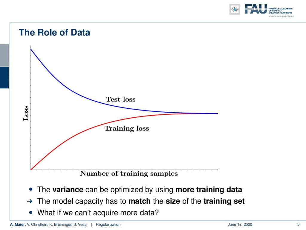
So let’s have a look at the role of data. Here, we plot the loss against the number of training samples and what you see is that the training loss increases with the number of training samples. It’s more difficult to learn a large data set than a small one. If you have a very small data set it may be very easy to memorize it entirely. The problem of a small data set is that it will not be very representative of the data that you’re actually interested in. So, the small data set model, of course, will have a high test loss. Now, by increasing the size of the data set, you increase the training loss as well but the test error goes down. This is what we’re interested in. We want to build general models that really work on unseen data. This is a very important property. It is also the reason why we need so much data and also why big companies are interested in getting so much data and storing it on their servers. Technically, we can optimize the variance by using more training data. So, we can create models of higher capacity but then we also need more training data but in the long run, this is likely to give us very low test errors. Also, the model capacity has to match the size of the training data set. If you have a too high capacity, it will just create a really bad over fit and your model will not be very good on unseen data. Now, the question is, of course, what if we can’t get more data?
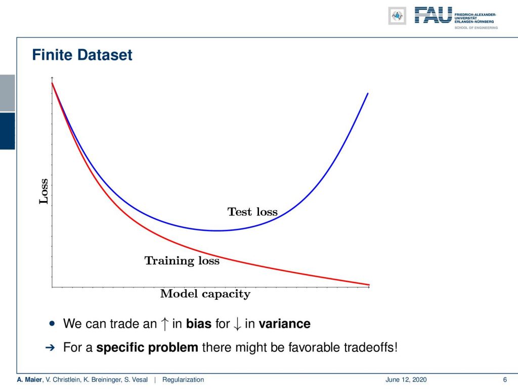
Let’s say you’re in a domain where we have limited data. Then, of course, you are in trouble. Let’s study these effects with a fixed data set size. So, on a finite data set, you make the following observations: if you increase the model capacity, your training loss will go down. Of course, with a higher capacity, you can memorize more of the training data set. This is the brute force way of solving a learning problem by just memorizing everything. The problem is you produce a bad over fit at some point. In the beginning, increasing the model capacity will also reduce the test loss. At some point when you go into the overfit, the test loss will increase, and if the test loss increases you are essentially at the point where you’re overfitting. Later in this class, we will look into the idea of using a validation data set that we take out from the training data set in order to produce a surrogate of the test loss. So, we will talk about this in a couple of lectures. What we can see here is that we can trade an increase in bias for a reduction in variance.
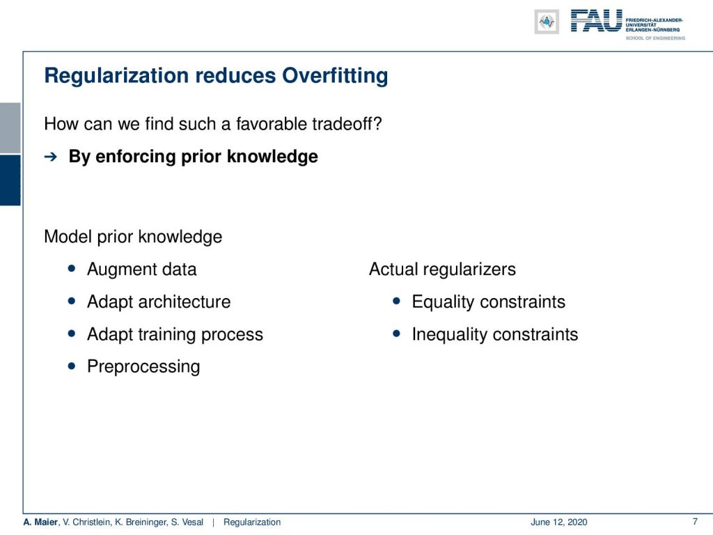
For a specific problem, there might be favorable trade-offs. Generally, the idea of regularization now is to reduce overfitting. Where does the idea come from? Well, we enforce essentially prior knowledge. One approach is data augmentation. You can adapt the architecture because you know something about the problem, you can adapt the training processes, and you can do pre-processing, and so on so. There are a lot of additional steps that can be taken in order to incorporate prior knowledge. The actual regularizes can also be used and there then be augmented into the loss functions and they typically constrain the solutions to equality constraints or inequality constraints. So, we will also have a short look at these solutions.
This already brings us to the end of this lecture. Next time, we will look into the classical regularization methods used in neural networks and machine learning. I’m looking forward to seeing you again in the next session!
If you liked this post, you can find more essays here, more educational material on Machine Learning here, or have a look at our Deep Learning Lecture. I would also appreciate a clap or a follow on YouTube, Twitter, Facebook, or LinkedIn in case you want to be informed about more essays, videos, and research in the future. This article is released under the Creative Commons 4.0 Attribution License and can be reprinted and modified if referenced.
Links
Link – for details on Maximum A Posteriori estimation and the bias-variance decomposition
Link – for a comprehensive text about practical recommendations for regularization
Link – the paper about calibrating the variances
References
[1] Sergey Ioffe and Christian Szegedy. “Batch Normalization: Accelerating Deep Network Training by Reducing Internal Covariate Shift”. In: Proceedings of The 32nd International Conference on Machine Learning. 2015, pp. 448–456.
[2] Jonathan Baxter. “A Bayesian/Information Theoretic Model of Learning to Learn via Multiple Task Sampling”. In: Machine Learning 28.1 (July 1997), pp. 7–39.
[3] Christopher M. Bishop. Pattern Recognition and Machine Learning (Information Science and Statistics). Secaucus, NJ, USA: Springer-Verlag New York, Inc., 2006.
[4] Richard Caruana. “Multitask Learning: A Knowledge-Based Source of Inductive Bias”. In: Proceedings of the Tenth International Conference on Machine Learning. Morgan Kaufmann, 1993, pp. 41–48.
[5] Andre Esteva, Brett Kuprel, Roberto A Novoa, et al. “Dermatologist-level classification of skin cancer with deep neural networks”. In: Nature 542.7639 (2017), pp. 115–118.
[6] C. Ding, C. Xu, and D. Tao. “Multi-Task Pose-Invariant Face Recognition”. In: IEEE Transactions on Image Processing 24.3 (Mar. 2015), pp. 980–993.
[7] Li Wan, Matthew Zeiler, Sixin Zhang, et al. “Regularization of neural networks using drop connect”. In: Proceedings of the 30th International Conference on Machine Learning (ICML-2013), pp. 1058–1066.
[8] Nitish Srivastava, Geoffrey E Hinton, Alex Krizhevsky, et al. “Dropout: a simple way to prevent neural networks from overfitting.” In: Journal of Machine Learning Research 15.1 (2014), pp. 1929–1958.
[9] R. O. Duda, P. E. Hart, and D. G. Stork. Pattern Classification. John Wiley and Sons, inc., 2000.
[10] Ian Goodfellow, Yoshua Bengio, and Aaron Courville. Deep Learning. http://www.deeplearningbook.org. MIT Press, 2016.
[11] Yuxin Wu and Kaiming He. “Group normalization”. In: arXiv preprint arXiv:1803.08494 (2018).
[12] Kaiming He, Xiangyu Zhang, Shaoqing Ren, et al. “Delving deep into rectifiers: Surpassing human-level performance on imagenet classification”. In: Proceedings of the IEEE international conference on computer vision. 2015, pp. 1026–1034.
[13] D Ulyanov, A Vedaldi, and VS Lempitsky. Instance normalization: the missing ingredient for fast stylization. CoRR abs/1607.0 [14] Günter Klambauer, Thomas Unterthiner, Andreas Mayr, et al. “Self-Normalizing Neural Networks”. In: Advances in Neural Information Processing Systems (NIPS). Vol. abs/1706.02515. 2017. arXiv: 1706.02515.
[15] Jimmy Lei Ba, Jamie Ryan Kiros, and Geoffrey E Hinton. “Layer normalization”. In: arXiv preprint arXiv:1607.06450 (2016).
[16] Nima Tajbakhsh, Jae Y Shin, Suryakanth R Gurudu, et al. “Convolutional neural networks for medical image analysis: Full training or fine tuning?” In: IEEE transactions on medical imaging 35.5 (2016), pp. 1299–1312.
[17] Yoshua Bengio. “Practical recommendations for gradient-based training of deep architectures”. In: Neural networks: Tricks of the trade. Springer, 2012, pp. 437–478.
[18] Chiyuan Zhang, Samy Bengio, Moritz Hardt, et al. “Understanding deep learning requires rethinking generalization”. In: arXiv preprint arXiv:1611.03530 (2016).
[19] Shibani Santurkar, Dimitris Tsipras, Andrew Ilyas, et al. “How Does Batch Normalization Help Optimization?” In: arXiv e-prints, arXiv:1805.11604 (May 2018), arXiv:1805.11604. arXiv: 1805.11604 [stat.ML].
[20] Tim Salimans and Diederik P Kingma. “Weight Normalization: A Simple Reparameterization to Accelerate Training of Deep Neural Networks”. In: Advances in Neural Information Processing Systems 29. Curran Associates, Inc., 2016, pp. 901–909.
[21] Xavier Glorot and Yoshua Bengio. “Understanding the difficulty of training deep feedforward neural networks”. In: Proceedings of the Thirteenth International Conference on Artificial Intelligence 2010, pp. 249–256.
[22] Zhanpeng Zhang, Ping Luo, Chen Change Loy, et al. “Facial Landmark Detection by Deep Multi-task Learning”. In: Computer Vision – ECCV 2014: 13th European Conference, Zurich, Switzerland, Cham: Springer International Publishing, 2014, pp. 94–108.