The Elman Cell
These are the lecture notes for FAU’s YouTube Lecture “Deep Learning“. This is a full transcript of the lecture video & matching slides. We hope, you enjoy this as much as the videos. Of course, this transcript was created with deep learning techniques largely automatically and only minor manual modifications were performed. If you spot mistakes, please let us know!
Welcome everybody to a new session of deep learning. Today we want to look into sequential learning and in particular recurrent neural networks. So far, we only had simple feed-forward networks where we had essentially a fixed size input and would then generate a classification result like “cat”, “dog”, or “hamster”.
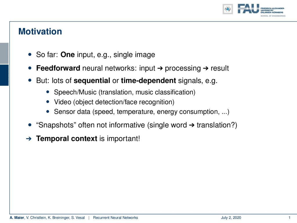
If we have sequences like audio, speech, language, or videos that have a temporal context, the techniques that we’ve seen so far are not that very well suited. So, we’re interested now is looking into methods that will be applicable to very long input sequences. Recurrent neural networks (RNNs) are exactly one method to actually do so. After a first review of the motivation, we’ll go ahead and look into simple recurrent neural networks. Then, we’ll introduce the famous long short-term memory units followed by gated recurrent units. After that, we will compare these different techniques and discuss a bit the pros and cons. Finally, we will talk about sampling strategies for our RNNs. Of course, this is way too much for a single video. So, we will talk about the different topics in individual short videos. So, let’s look at the motivation. Well, we had one input for one single image but this is not so great for sequential or time-dependent signals such as speech, music, video, or other sensor data. You could even talk about very simple sensors that measure energy consumption. So snapshots with a fixed length are often not that informative. If you look at a single word you probably have trouble getting the right translation because the context matters. The temporal context is really important and it needs to be modeled appropriately.
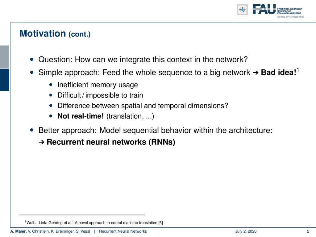
The question is now: “How can we integrate this context into the network?” The simple approach would be to feed the whole sequence to a big network. This is potentially a bad idea because we have inefficient memory usage. It’s difficult to train or even impossible to train and we would never figure out the difference between spatial and temporal dimensions. We would just handle all the same. Actually maybe it’s not such a bad idea. For rather simple tasks, as you can see in [6] because they actually investigated this and found quite surprising results with CNNs. Well, one problem that you have of course is it won’t be real-time because you need the entire sequence for the processing. So, the approach that we are suggesting in this and the next couple of videos is to model sequential behavior within the architecture and that gives rise to recurrent neural networks.
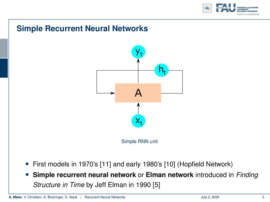
So let’s have a look at the simple recurrent neural networks. The main idea is that you introduce a hidden state h subscript t that is carried on over time. So this can be changed but it is essentially connecting back to the original cell A. So, A is our recurrent cell and it has this hidden state that is somehow allowing us to encode what the current temporal information has brought to us. Now, we have some input x subscript t and this will then generate some output y subscript t and by the way, the first models were from the 1970s and early 1980s like Hopfield networks. Here, we will stick with the simple recurrent neural network or Elman network as introduced in [5].
Now, feed-forward networks only feed information forward. So with recurrent networks, in contrast, we can now model loops, we can model memory and experience, and we learn sequential relationships. So, we can provide continuous predictions as the data comes in. This enables us to process everything in real-time.
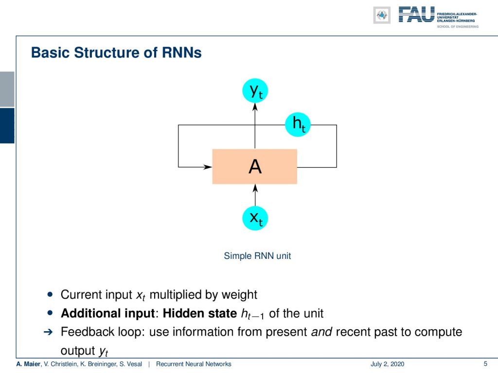
Now, this is again our basic recurrent neural network where we have some input x that is multiplied with some weight. Then, we have the additional input, the hidden state from the previous configuration, and we have essentially a feedback loop where you use the information from the present and the recent past.
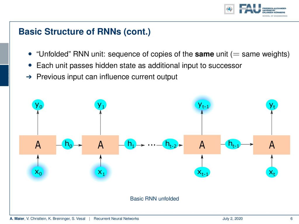
To compute the output y subscript t, we essentially end up with an unfolded structure. So, if you want to evaluate the recurrent unit, what you do is you start with some x₀ that you process with your unit. This generates a new result y₀ and the new hidden state h₀. Now, h₀ is fed forward to the next instance of where essentially the weights are coupled. So we have exactly the same copy of the same unit in the next time state but h is, of course, different. So now, we feed in x₁ process generate y₁ and produce a new hidden state h₁ and so on. We can do that until we are at the end of the sequence so each unit passes on the hidden state as an additional input to the successor. This means that the previous input can have an influence on the current output because if we’ve seen x₀ and x₁, they can have an influence on y subscript (t-1), just because we have encoded the information that we observed x₀ and x₁ in the hidden state. So, the hidden state allows us to store information and carry it through the entire network to a certain period of time where we then want to choose a specific action.
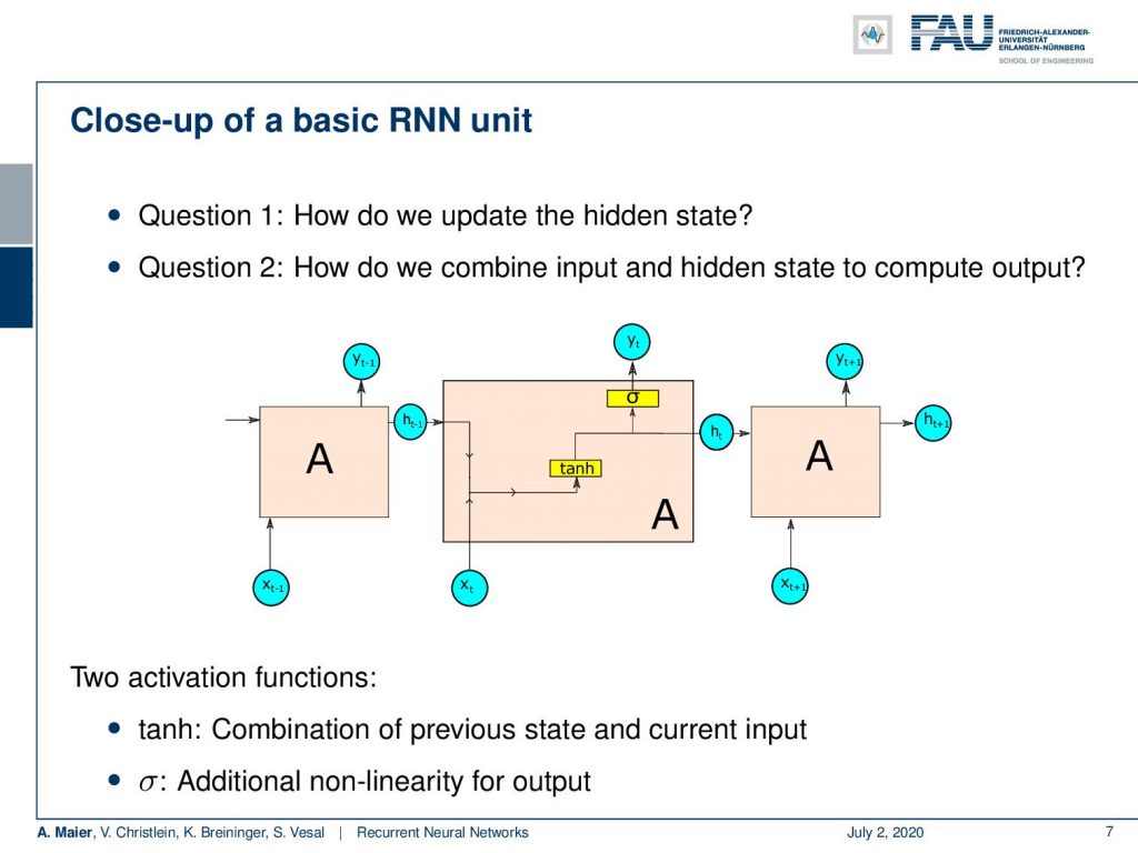
So now, the basic question is “How do we update the hidden state?” and the second question is “How do we combine input and hidden state to compute the output?” So, we do that opening the cell and looking inside. What you see here is that we essentially concatenate the hidden state with the new input then feed it to a non-linearity, here, a hyperbolic tangent. This produces a new state and from the new state, we’re generating the new output with a sigmoid function. Then, we hand the new hidden state over to the next instance of the same cell. So, we have two activation functions: the hyperbolic tangent for combining the previous state and the current state and the sigmoid non-linearity for generating the output.
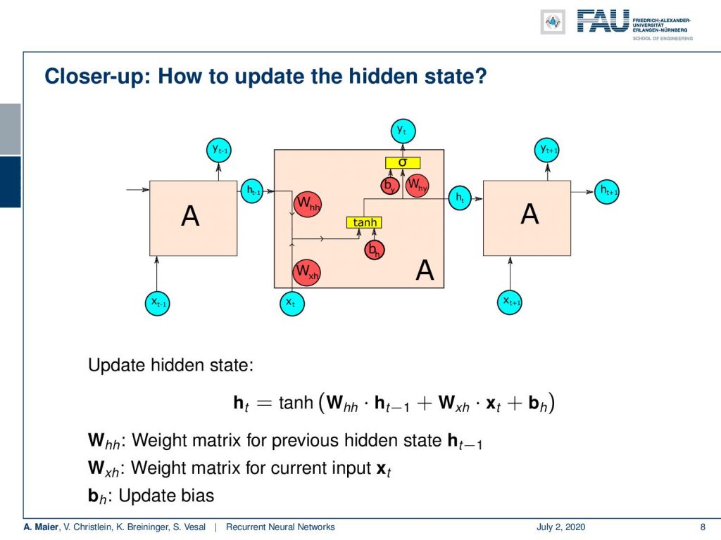
In order to do so, of course, we need weight matrices and those weight matrices are essentially depicted here in red. We can look at them in a little more detail if we want to update the hidden state. This is essentially the hidden state transition matrix W subscript hh times the last hidden state plus the input to hidden state conversion matrix W subscript xh times x subscript t plus the bias. This is then fed to the non-linearity which then produces the new hidden state.
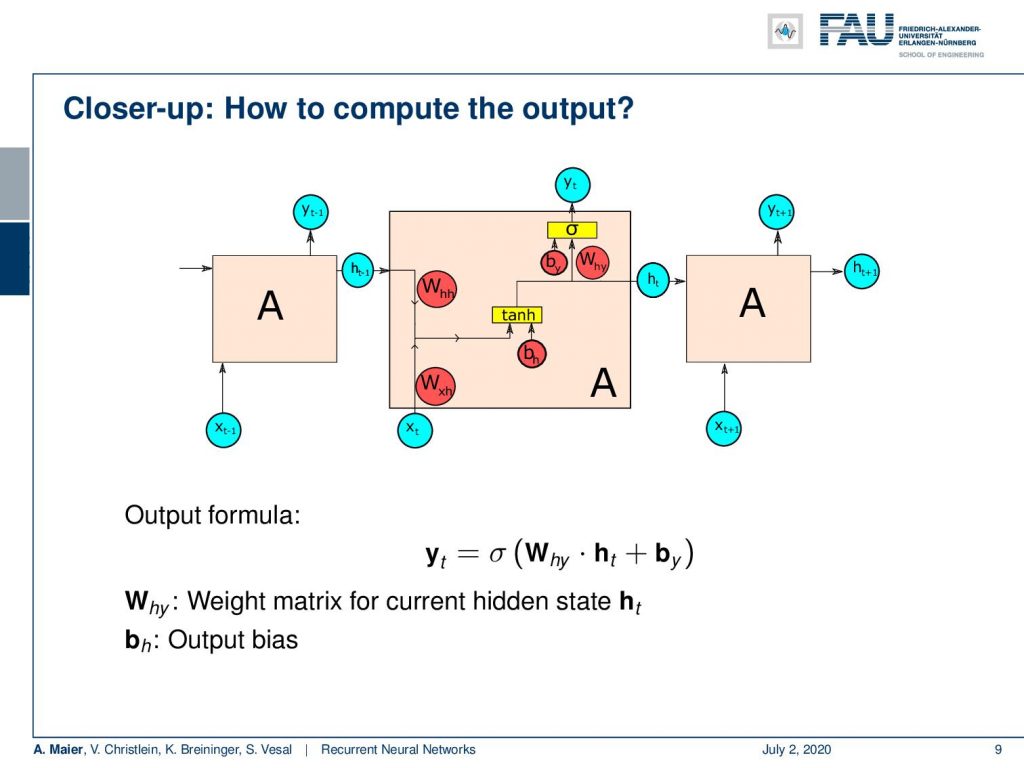
Ok, so how can we compute the output? Well, we have produced a new hidden state which means that we now just have another transition matrix that produces a preliminary output from the hidden state. So we have this new W subscript hy that is taking h subscript t and some bias and feeds it to the sigmoid function to produce the final output.
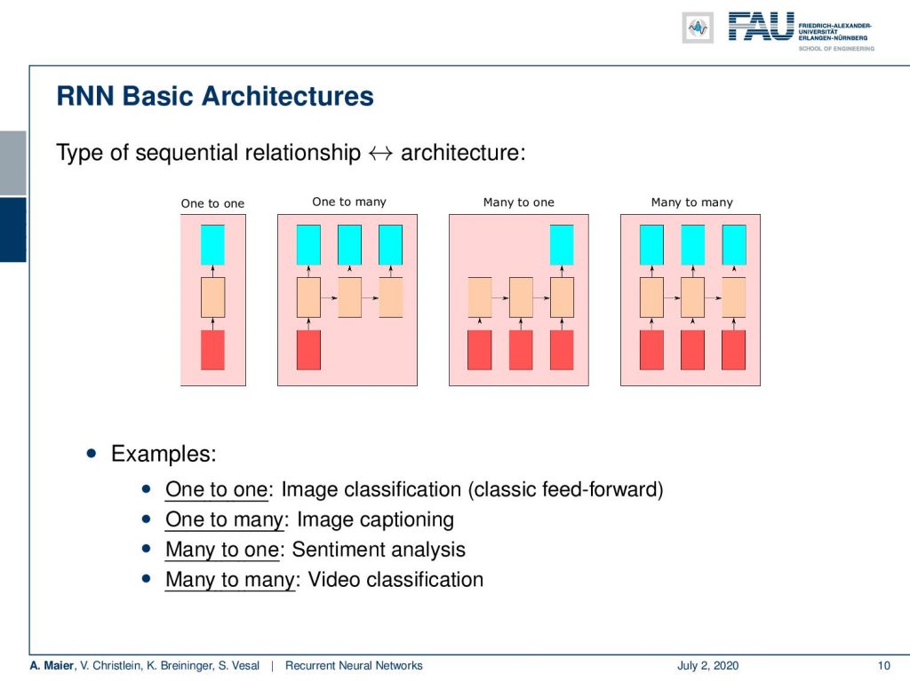
If we stick to this architecture, we can then essentially realize many different types of architectures. This is determined by the setup of the architecture. So, we can do one to one mapping where we have one input cell and essentially one output cell, but you can also do one too many, many to one, or you can even many do many. So example of one-to-one is image classification. It’s essentially classic feedforward. One-to-many would be image captioning. Many-to-one would be sentiment analysis where you need to observe a certain sequence in order to figure out what sentiment is going on in this situation. Many-to-many is video classification.
Of course, we can also think about deep RNNS. So far, we only have one hidden layer and we can just use our recurring model which is why we need to go deeper. In this case, it’s more like “Yo, dawg I heard you like RNNs, so I put an RNN on your RNN on your RNN.”
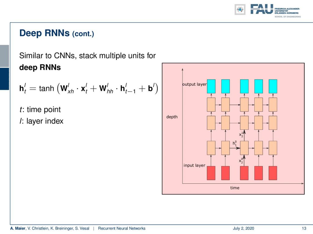
Well, what emerges from this is architectures like this one here. We simply stack multiple hidden units for deep RNNs. So, we can, of course, stack Elman cells on our Elman cells. Then, we would be essentially decoding this using inputs over time, decode them with multiple RNN cells, and produce multiple outputs over time. So, this then gives us access to deep elements.
Ok. So, this is the simple introduction to deep RNNs and recurrent neural networks. In the next video, we want to go into a little bit more detail and actually see how the training is done and the actual update equations in order to perform the training. So, I hope you like this video and see you in the next one!
If you liked this post, you can find more essays here, more educational material on Machine Learning here, or have a look at our Deep LearningLecture. I would also appreciate a follow on YouTube, Twitter, Facebook, or LinkedIn in case you want to be informed about more essays, videos, and research in the future. This article is released under the Creative Commons 4.0 Attribution License and can be reprinted and modified if referenced.
RNN Folk Music
FolkRNN.org
MachineFolkSession.com
The Glass Herry Comment 14128
Links
Character RNNs
CNNs for Machine Translation
Composing Music with RNNs
References
[1] Dzmitry Bahdanau, Kyunghyun Cho, and Yoshua Bengio. “Neural Machine Translation by Jointly Learning to Align and Translate”. In: CoRR abs/1409.0473 (2014). arXiv: 1409.0473.
[2] Yoshua Bengio, Patrice Simard, and Paolo Frasconi. “Learning long-term dependencies with gradient descent is difficult”. In: IEEE transactions on neural networks 5.2 (1994), pp. 157–166.
[3] Junyoung Chung, Caglar Gulcehre, KyungHyun Cho, et al. “Empirical evaluation of gated recurrent neural networks on sequence modeling”. In: arXiv preprint arXiv:1412.3555 (2014).
[4] Douglas Eck and Jürgen Schmidhuber. “Learning the Long-Term Structure of the Blues”. In: Artificial Neural Networks — ICANN 2002. Berlin, Heidelberg: Springer Berlin Heidelberg, 2002, pp. 284–289.
[5] Jeffrey L Elman. “Finding structure in time”. In: Cognitive science 14.2 (1990), pp. 179–211.
[6] Jonas Gehring, Michael Auli, David Grangier, et al. “Convolutional Sequence to Sequence Learning”. In: CoRR abs/1705.03122 (2017). arXiv: 1705.03122.
[7] Alex Graves, Greg Wayne, and Ivo Danihelka. “Neural Turing Machines”. In: CoRR abs/1410.5401 (2014). arXiv: 1410.5401.
[8] Karol Gregor, Ivo Danihelka, Alex Graves, et al. “DRAW: A Recurrent Neural Network For Image Generation”. In: Proceedings of the 32nd International Conference on Machine Learning. Vol. 37. Proceedings of Machine Learning Research. Lille, France: PMLR, July 2015, pp. 1462–1471.
[9] Kyunghyun Cho, Bart Van Merriënboer, Caglar Gulcehre, et al. “Learning phrase representations using RNN encoder-decoder for statistical machine translation”. In: arXiv preprint arXiv:1406.1078 (2014).
[10] J J Hopfield. “Neural networks and physical systems with emergent collective computational abilities”. In: Proceedings of the National Academy of Sciences 79.8 (1982), pp. 2554–2558. eprint: http://www.pnas.org/content/79/8/2554.full.pdf.
[11] W.A. Little. “The existence of persistent states in the brain”. In: Mathematical Biosciences 19.1 (1974), pp. 101–120.
[12] Sepp Hochreiter and Jürgen Schmidhuber. “Long short-term memory”. In: Neural computation 9.8 (1997), pp. 1735–1780.
[13] Volodymyr Mnih, Nicolas Heess, Alex Graves, et al. “Recurrent Models of Visual Attention”. In: CoRR abs/1406.6247 (2014). arXiv: 1406.6247.
[14] Bob Sturm, João Felipe Santos, and Iryna Korshunova. “Folk music style modelling by recurrent neural networks with long short term memory units”. eng. In: 16th International Society for Music Information Retrieval Conference, late-breaking Malaga, Spain, 2015, p. 2.
[15] Sainbayar Sukhbaatar, Arthur Szlam, Jason Weston, et al. “End-to-End Memory Networks”. In: CoRR abs/1503.08895 (2015). arXiv: 1503.08895.
[16] Peter M. Todd. “A Connectionist Approach to Algorithmic Composition”. In: 13 (Dec. 1989).
[17] Ilya Sutskever. “Training recurrent neural networks”. In: University of Toronto, Toronto, Ont., Canada (2013).
[18] Andrej Karpathy. “The unreasonable effectiveness of recurrent neural networks”. In: Andrej Karpathy blog (2015).
[19] Jason Weston, Sumit Chopra, and Antoine Bordes. “Memory Networks”. In: CoRR abs/1410.3916 (2014). arXiv: 1410.3916.