Lecture Notes in Deep Learning: Loss and Optimization – Part 1

Classification and Regression Losses

These are the lecture notes for FAU’s YouTube Lecture “Deep Learning“. This is a full transcript of the lecture video & matching slides. We hope, you enjoy this as much as the videos. Of course, this transcript was created with deep learning techniques largely automatically and only minor manual modifications were performed. If you spot mistakes, please let us know!

Welcome everybody to deep learning! So, today we want to continue talking about the different losses and optimization. We want to go ahead and talk a bit about more details of these interesting problems. Let’s talk first about the loss functions first. Loss functions are generally used for different tasks and for different tasks you have different loss functions.

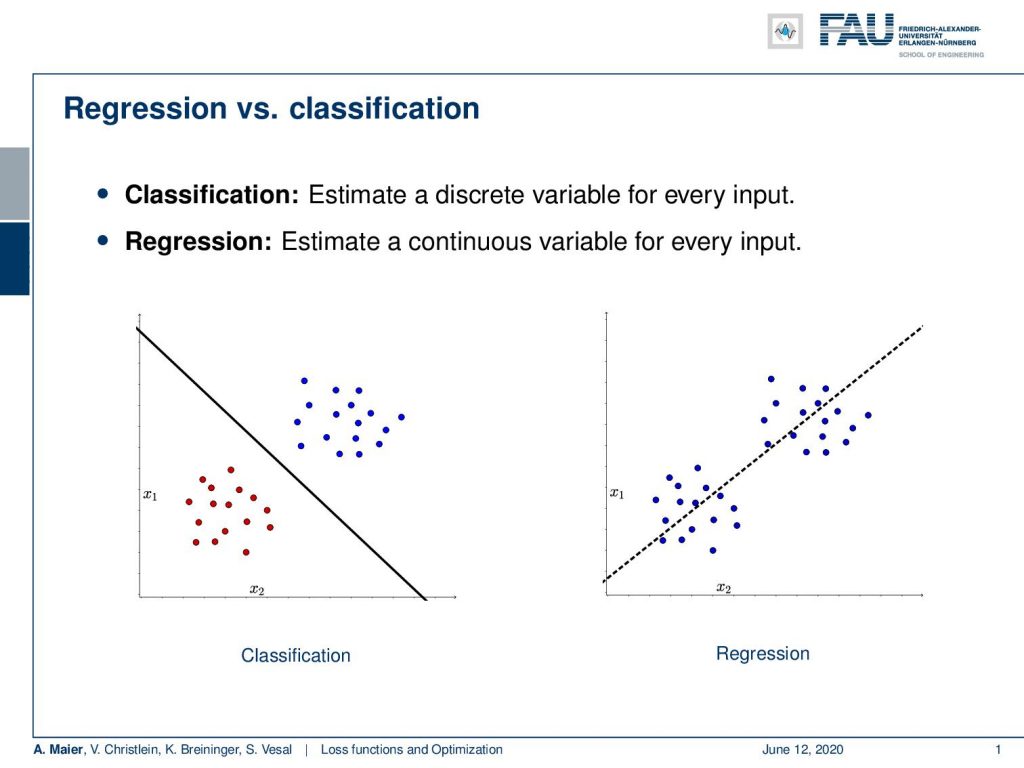
The two most important tasks that we are facing are regression and classification. So in classification, you want to estimate a discrete variable for every input. This means that you want to essentially decide in this two-class problem here on the left whether it’s blue or red dots. So, you need to model a decision boundary.

In regression, the idea is that you want to model a function that explains your data. So, you have some input function let’s say x₂ and you want to predict x₁ from it. To do so, you compute a function that will produce the appropriate value of x₁ for any given x₂. Here in this example, you can see this is a line fit.

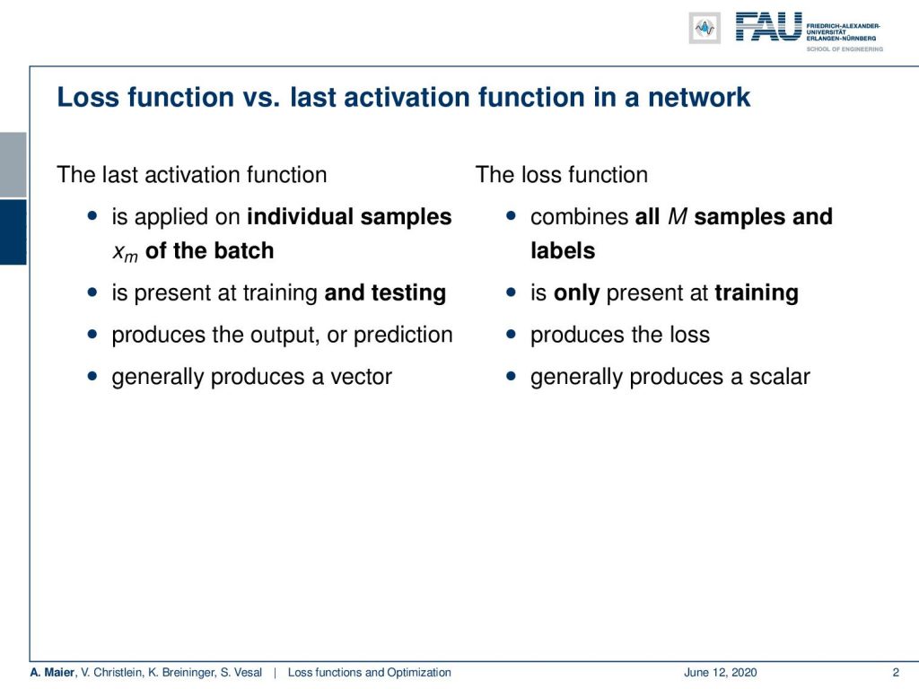
We talked about activation functions, last activation as softmax, and cross-entropy loss. Somehow, we combined them and obviously there’s a difference between the last activation function in our network and the loss function. The last activation function is applied to the individual samples x each of the batch. It will also be present at training and testing time. So, the last activation function will become part of the network and will remain there to produce the output / the prediction. It generally produces a vector.

Now, the loss function combines all M samples and labels. In their combination, they produce a loss that describes how good the fit is. So, it’s only present during training time and the loss is generally a scalar value that describes how good the fit is. So, you only need it during training time.

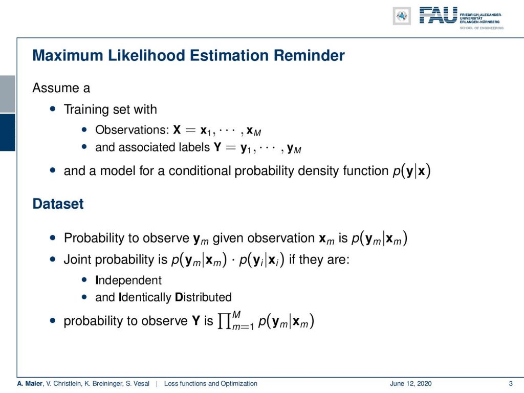
Interestingly, many of those loss functions can be put in a probabilistic framework. This leads us to maximum likelihood estimation. In maximum likelihood estimation – just as a reminder – we consider everything to be probabilistic. So, we have a set of observations X that consists of individual observations. Then, we have associated labels. They also stem from some distribution and the observations are denoted as Y. Of course, we need a conditional probability density function that describes us somehow how y and x are related. In particular, we can compute the probability for y given some observation x. This will be very useful for example if we want to decide on a specific class. Now, we have to somehow model this data set. They are drawn from some distribution and the joint probability for the given data set can then be computed as a product over the individual conditional probabilities. Of course, if they’re independent and identically distributed, you can simply write this up as a large product over the entire training data set. So, you end up with this product over all M samples, where it’s just a product of the conditionals. This is useful because we can determine the best parameters by maximizing the joint probability over the entire training data set. We have to do it by evaluating this large product.

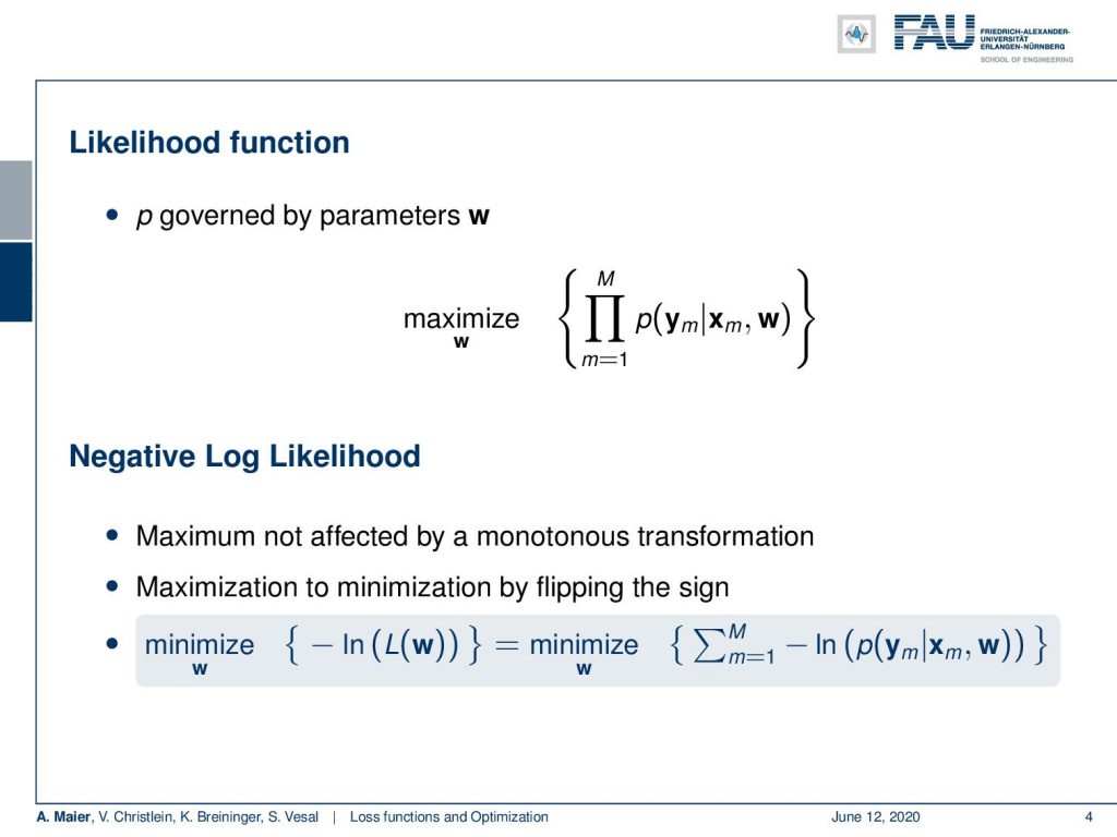
Now, this large product has a couple of problems. In particular, if we have high and low values, they may cancel out very quickly. So, it may be interesting to transform the entire problem into the logarithmic domain. Because the logarithm is a monotonous transformation, it doesn’t change the position of the maximum. Hence, we can use the log function and a negative sign to flip the maximization into a minimization. Instead of looking at the likelihood function, we can look at the negative log-likelihood function. Then, our large product is suddenly a sum over all the observations times the negative logarithm of the conditional probabilities.

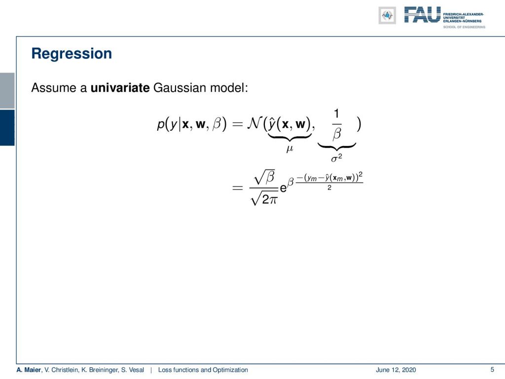
Now, we can look at a univariate gaussian model. So, now we are one dimensional again and we can model this with a normal distribution where we would then choose the output of our network as the expected value and 1/β as the standard deviation. If we do so, we can find the following formulation: Square root of beta over square root of 2 pi times the exponential function of minus beta times the label minus the prediction to the power of 2 divided by 2.

Okay so let’s go ahead and put this into our log-likelihood function. Remember this is really something, you should know in the oral exam. Everybody needs to know the normal distribution and everybody needs to be able to convert this kind of universe Gaussian distribution into a loss function. If we do so, you will see that we can use the logarithm. It comes in very handy because it allows us to split the product here. Then, we also see that the logarithm cancels out with the exponential function. We simply get this beta over 2 times y subscript m minus y hat subscript m to the power of 2. We can simplify the first term further by applying the logarithm and pulling out the square root 2 pi. Then, we see that the sum over the first two terms is not depending on m, so we can simply multiply by M in order to get rid of the sum and move the sum only to the last term.

Now, you can see that only the last part here actually depends on w. Everything else doesn’t even contain w. So, if we seek to optimize towards w, we can simply neglect the first two parts. Then, we end up only with the part here on the right-hand side. You see that if we now assume β to be 1, we end up exactly with 1/2 and the sum over the square root of the differences. This is nothing else than the L2 norm. If you would write it in vector notation, you end up with this here. Of course, this is equivalent to a multi-dimensional Gaussian distribution with uniform variance.

Okay, so well there’s not just L2-losses. There’s also L1 losses. So, we can also replace those, and we will look at some properties of different L norms in a couple of videos as well. It’s generally a very nice approach and it corresponds to minimizing the expected misclassification probability. It may cause slow convergence, because they don’t penalize heavy misclassified probabilities, but they may be advantageous in extreme label noise.

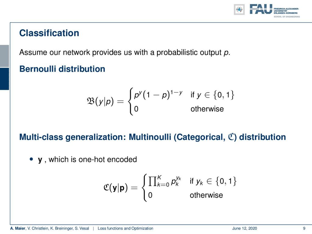
Now, let’s assume now let’s assume that we want to classify. Then, our network would provide us with some probabilistic output p. Let’s say, we classify only into two classes. Then, we can model this as a Bernoulli distribution where we have classes zero and one. Of course, the probability of the other class is simply one minus p. This then gives us the probability distribution pʸ times (1 – p)¹⁻ʸ. Typically, we don’t have only two classes. This means we need to generalize to the multinulli or categorical distribution. Then y is typically modeled again one-hot encoded vector. We can then write down the categorical distribution as the product over all the classes of the probability for each class to the power of the ground truth label which is either zero or one.

Let’s look at an example of a categorical distribution. The example that we want to take here is a Bernoulli trial a coin flip. We encode head as (1 0)ᵀ and tail as (0 1)ᵀ. Then, we have an unfair coin and this unfair coin prefers tails with a probability of 0.7. Its likelihood for heads is 0.3. Then, we observe the true label y as tails. Now, we can use the above equation and plug those observations in. This means we get 0.3 to the power of 0 and 0.7 to the power of 1. Something to the power of 0 always equals to 1. Then 0.7 to the power of 1 is of course 0.7. This gives us 0.7 and this then means that the probability to observe tails for our unfair coin is 70%.

We can always use the softmax function within the network to convert everything into probabilities. Now, we can look at how this behaves with our categorically distributed system. Here, we simply replace our conditional with the categorical distribution. This then gives us a negative log-likelihood function. Again what we’re doing here is of high relevance for the oral exam. So everybody should be able to explain how to come from a probabilistic assumption to the respective loss function using the categorical distribution. So here, we again apply the negative log-likelihood. We plug in the definition of the categorical distribution which is simply the product over all our y subscript k hat to the power of the ground truth label. This can be further simplified because the product can be converted into a sum by moving in the logarithm. If we do so, you can see that the power of the ground truth label can actually be pulled in front of the logarithm. We see that we exactly end up with cross-entropy. Now, if you use the trick with the one-hot encoding again, you can see that we exactly end up with the cross-entropy loss where we have the sum over the entire set of observations times the logarithm of the output at exactly the position where our ground truth label was 1. Hence, we neglect all the other terms in the sum of the classes.

Interestingly, this can also be put in relation to the Kullback Leibler (KL) Divergence. KL divergence is a very common construct that you find in many machine learning papers. Here, you can see the definition. We essentially have an integral over the entire domain of x. It’s integrating the probability of p(x) times the logarithm of p(x) divided by q(x). q(x) is the reference distribution that you want to compare to. Now, you can see that you can split the two into two parts using the property of the logarithm. So, we get the minus part on the right-hand-side which is the cross-entropy. The left-hand side is simply the entropy. So, we can see that this training process is essentially identical to minimizing the cross-entropy. So, in order to minimize the KL divergence, we can minimize the cross-entropy. You should keep that in mind this kind of relationship appears very often in machine learning papers. So you will find them easier to understand if you have these things in the back of your mind.

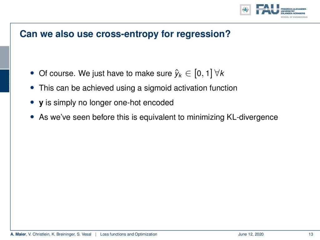
Now, can we use cross-entropy for regression? Well, yes we can do that of course. But you have to make sure that your predictions are going to be in the domain of [0, 1] for all of your classes. You can for example do this with a sigmoid activation function. Then you have to be careful because in regression typically you’re no longer one-hot encoded. So, this is something that you have to deal with appropriately. As seen before, this loss is equivalent to minimizing the KL divergence.

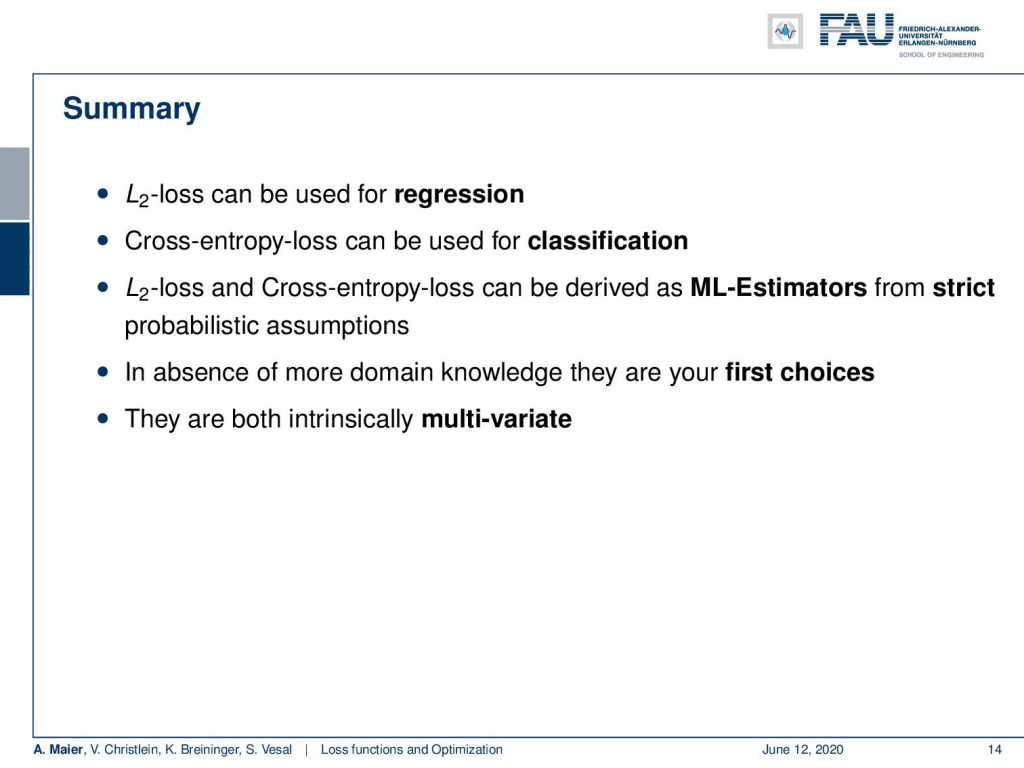
Let’s summarize what we’ve seen so far. So L2 loss is typically used for regression. Cross-entropy loss is typically used for classification typically in combination with one-hot encoding. Of course, you can derive them from ML estimators from strict probabilistic assumptions. So what we’re doing here is completely in line with probability theory. In the absence of more domain knowledge, these are our first choices. If you have additional domain knowledge then, of course, it’s a good idea to use it to build a better estimator. The cross-entropy loss is intrinsically multivariate. So, we are not just stuck with two-class problems. We can go to multi-dimensional regression and classification problems as well.

Next time in deep learning, we want to go into some more details about loss functions and in particular, we want to highlight the hinge loss. It is a very important loss function because it allows you to embed constraints. We will see that there are also some relations to classical machine learning and pattern recognition, in particular, the support vector machine. So I hope you enjoyed this video and I am looking forward to seeing you in the next one”!

If you liked this post, you can find more essays here, more educational material on Machine Learning here, or have a look at our Deep Learning Lecture. I would also appreciate a clap or a follow on YouTube, Twitter, Facebook, or LinkedIn in case you want to be informed about more essays, videos, and research in the future. This article is released under the Creative Commons 4.0 Attribution License and can be reprinted and modified if referenced.

References

[1] Christopher M. Bishop. Pattern Recognition and Machine Learning (Information Science and Statistics). Secaucus, NJ, USA: Springer-Verlag New York, Inc., 2006.
[2] Anna Choromanska, Mikael Henaff, Michael Mathieu, et al. “The Loss Surfaces of Multilayer Networks.” In: AISTATS. 2015.
[3] Yann N Dauphin, Razvan Pascanu, Caglar Gulcehre, et al. “Identifying and attacking the saddle point problem in high-dimensional non-convex optimization”. In: Advances in neural information processing systems. 2014, pp. 2933–2941.
[4] Yichuan Tang. “Deep learning using linear support vector machines”. In: arXiv preprint arXiv:1306.0239 (2013).
[5] Sashank J. Reddi, Satyen Kale, and Sanjiv Kumar. “On the Convergence of Adam and Beyond”. In: International Conference on Learning Representations. 2018.
[6] Katarzyna Janocha and Wojciech Marian Czarnecki. “On Loss Functions for Deep Neural Networks in Classification”. In: arXiv preprint arXiv:1702.05659 (2017).
[7] Jeffrey Dean, Greg Corrado, Rajat Monga, et al. “Large scale distributed deep networks”. In: Advances in neural information processing systems. 2012, pp. 1223–1231.
[8] Maren Mahsereci and Philipp Hennig. “Probabilistic line searches for stochastic optimization”. In: Advances In Neural Information Processing Systems. 2015, pp. 181–189.
[9] Jason Weston, Chris Watkins, et al. “Support vector machines for multi-class pattern recognition.” In: ESANN. Vol. 99. 1999, pp. 219–224.
[10] Chiyuan Zhang, Samy Bengio, Moritz Hardt, et al. “Understanding deep learning requires rethinking generalization”. In: arXiv preprint arXiv:1611.03530 (2016).

Category: Lecture Notes in Deep Learning