
Deep Design Patterns
These are the lecture notes for FAU’s YouTube Lecture “Deep Learning“. This is a full transcript of the lecture video & matching slides. We hope, you enjoy this as much as the videos. Of course, this transcript was created with deep learning techniques largely automatically and only minor manual modifications were performed. Try it yourself! If you spot mistakes, please let us know!

Welcome back to deep learning! This is it. This is the final lecture. So today, I want to show you a couple of more applications of this known operator paradigm and also some ideas where I believe future research could actually go to. So, let’s see what I have here for you. Well, one thing that I would like to demonstrate is the simplified modern hearing aid pipeline. This is a collaboration with a company that is producing hearing aids and they typically have a signal processing pipeline where you have two microphones. They collect some speech signals. Then, this is run through an analysis filter bank. So, this is essentially a short-term Fourier transform. This is then run through a directional microphone in order to focus on things that are in front of you. Then, you use noise reduction in order to get better intelligibility for the person who is wearing the hearing aid. This is followed by an automatic gain control and using the gain control you then do a synthesis of the frequency analysis back to a speech signal that is then played back on a loudspeaker within the hearing aid. So, there’s also a recurrent connection because you want to suppress feedback loops. This kind of pipeline, you can find in modern-day hearing aids of various manufacturers. Here, you see some examples and the key problem in all of this processing is here the noise reduction. This is the difficult part. All the other things, we know how to address with traditional signal processing. But the noise reduction is something that is a huge problem.
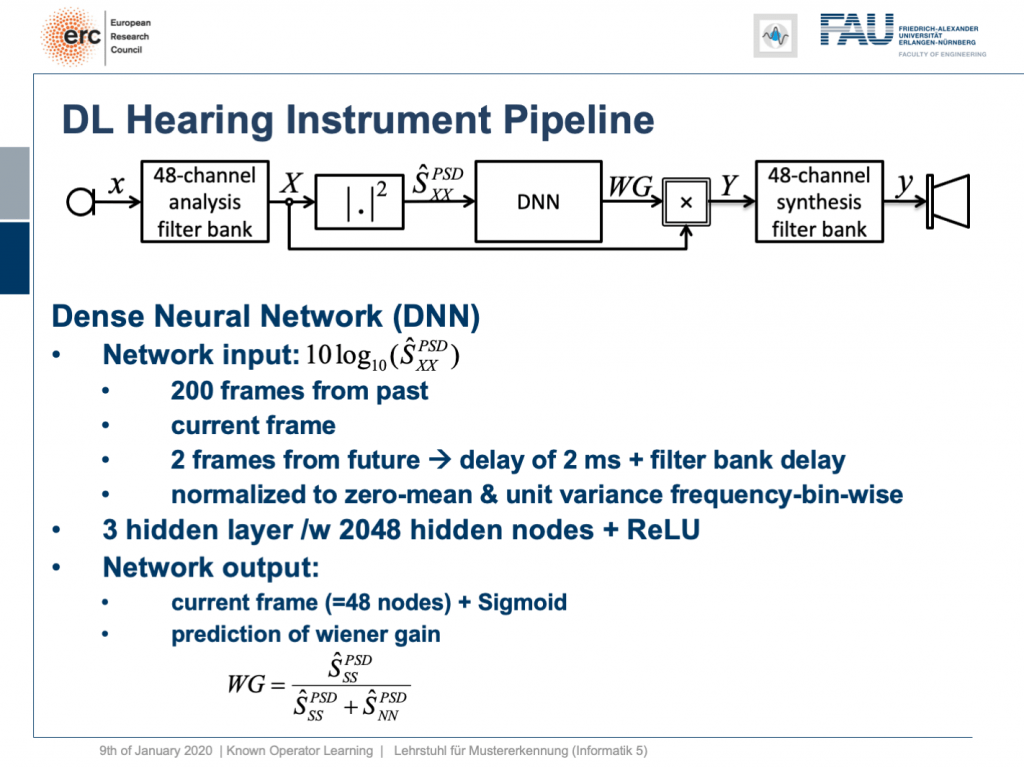
So, what can we do? Well, we can map this entire hearing aid pipeline onto a deep network. Onto a deep recurrent network and all of those steps can be expressed in terms of differentiable operations.
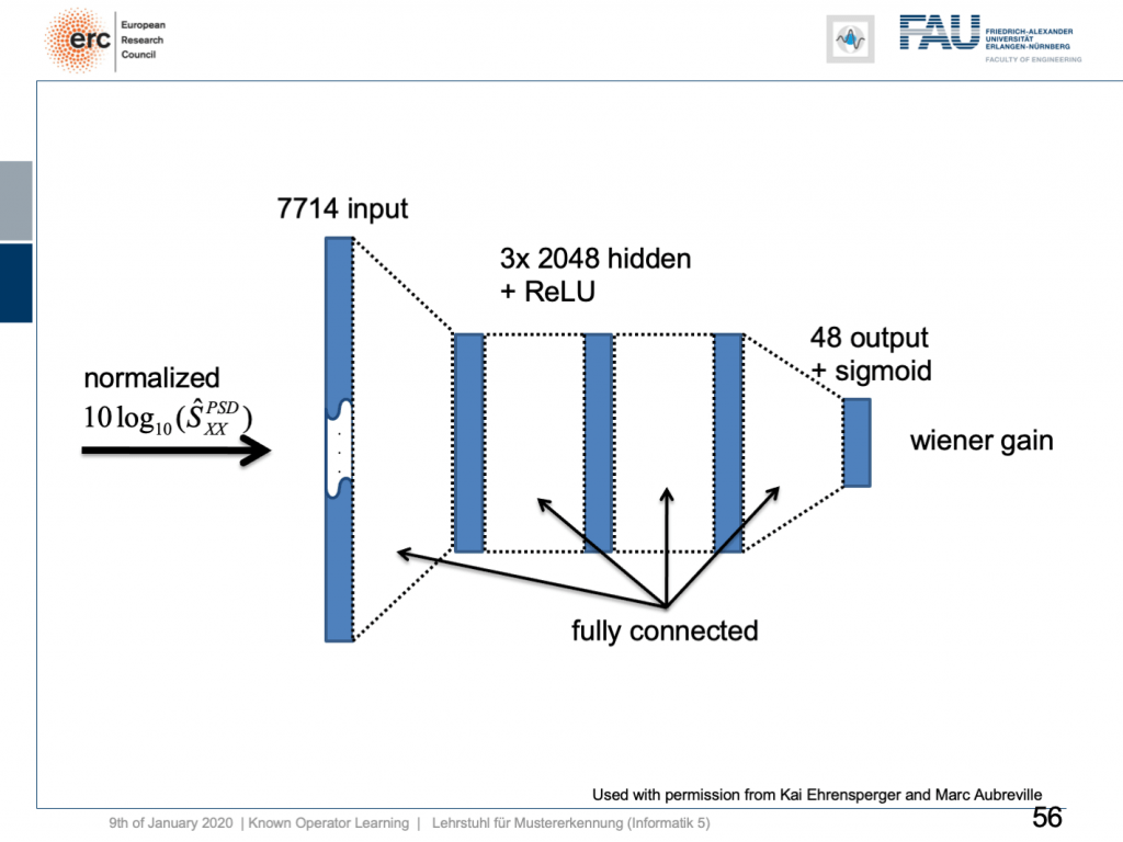
If we do so, we set up the following outline. Actually, our network here is not so deep because we only have three hidden layers but with 2024 hidden nodes and ReLUs. This is then used to predict the coefficients of a Wiener filter gain in order to suppress channels that have particular noises. So, this is the setup. We have an input of seven thousand seven hundred and fourteen nodes from our normalized spectrum. Then, this is run through three hidden layers. They are fully connected with ReLUs and in the end, we have some output that is 48 channels produced by the sigmoid producing our Wiener gain.
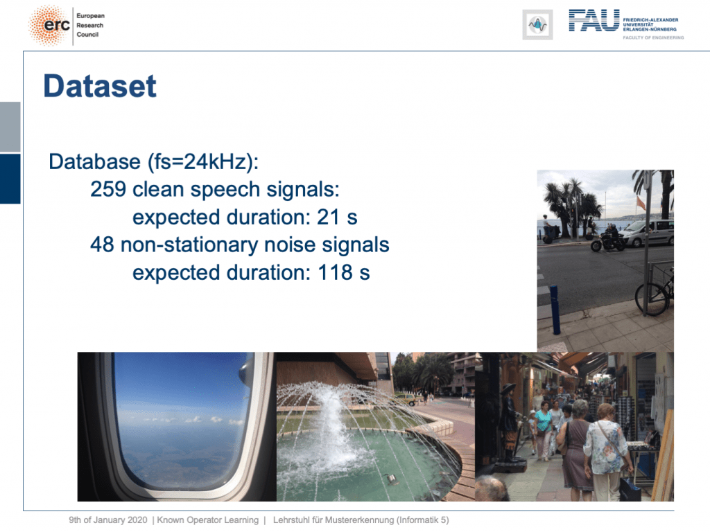
We evaluated this on some data set and here we had 259 clean speech signals. We then essentially had 48 non-stationary noise signals and we mixed them. So, you could argue what we’re essentially training here is a kind of recurrent autoencoder. Actually, a denoising autoencoder because as input we take the clean speech signal plus the noise and on the output, we want to produce the clean speech signal. Now, this is the example.
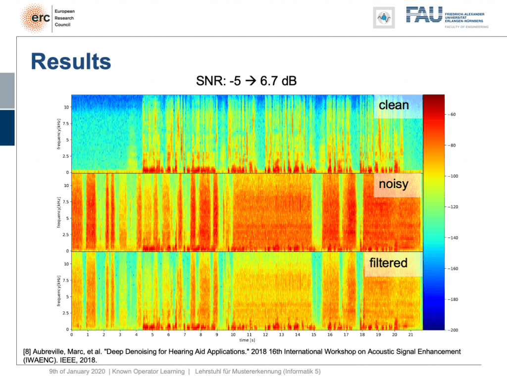
Let’s try a non-stationary noise pattern and this is an electronic drill. Also, note that the network has never heard an electronic drill before. This typically kills your hearing aid and let’s listen to the output. So, you can hear that the non-stationary noise is also very well suppressed. Wow. So, that’s pretty cool of course there are many more applications of this.

Let’s look into one more idea. Can we derive networks? So here, let’s say you have a scenario where you collect data in a format that you don’t like, but you know the formal equation between the data and the projection.
So, the example that I’m showing here is a cone-beam acquisition. This is simply a typical x-ray geometry. So, you take an X-ray and this is typically conducted in cone-beam geometry. Now, for the cone-beam geometry, we can describe it entirely using this linear operator as we’ve already seen in the previous video. So, we can express the relation between the object x our geometry A subscript CB and our projection p subscript CB. Now, the cone-beam acquisition is not so great because you have magnifications in there. So if you have something close to the source, it will be magnified more than an object closer to the detector. So, this is not so great for diagnosis. In othopedics, they would prefer parallel projections because if you have something, it will be orthogonally projected and it’s not magnified. This would be really great for diagnosis. You would have metric projections and you can simply measure int the projection and it would have the same size as inside the body. So, this would be really nice for diagnosis, but typically we can’t measure it with the systems that we have. So, in order to create this, you would have to create a full reconstruction of the object, doing a full CT scan from all sides, and then reconstruct the object and project it again. Typically in orthopedics, people don’t like slice volumes because they are far too complicated to read. But projection images are much nicer to read. Well, what can we do? We know the factor that connects two equations here is x. So we can simply solve this equation here and produce the solution with respect to x. Once, we have x and the matrix inverse here of A subscript CB times p subscript CB. Then, we simply would multiply it to our production image. But we are not interested in the reconstruction. We are interested in this projection image here. So, let’s plug it into our equation and then we can see that by applying this series of matrices we can convert our cone-beam projections into a parallel-beam projection p subscript PB. There’s no real reconstruction required. Only a kind of intermediate reconstruction is required. Of course, you don’t just acquire a single projection here. You may want to acquire a couple of those projections. Let’s say three or four projections but not thousands as you would in a CT scan. Now, if you look at this set of equations, we know all of the operations. So, this is pretty cool. But we have this inverse here and note that this is again a kind of reconstruction problem, an inverse of a large matrix that is sparse to a large extent. So, we still have a problem estimating this guy here. This is very expensive to do, but we are in the world of deep learning and we can just postulate things. So, let’s postulate that this inverse is simply a convolution. So, we can replace it by a Fourier transform a diagnoal matrix K and an inverse Fourier transform. Suddenly, I’m only estimating parameters of a diagonal matrix which makes the problem somewhat easier. We, can solve it in this domain and again we can use our trick that we have essentially defined a known operator net topology here. We can simply use it with our neural network methods. We use the backpropagation algorithm in order to optimize this guy here. We just use the other layers as fixed layers. By the way, this could also be realized for nonlinear formulas. So, remember as soon as we’re able to compute a subgradient, we can plug it into our network. So you can also do very sophisticated things like including a median filter for example.
Let’s look at an example here. We do the rebinning of MR projections in this case. We will do an acquisition in k-space and these are typically just parallel projections. Now, we’re interested in generating overlay for X-rays and x-rays we need the come-beam geometry. So, we take a couple of our projections and then rebin them to match exactly the come-beam geometry. The cool thing here is that we would be able to unite the contrasts from MR and X-ray in a single image. This is not straightforward. If you initialize with just the Ram-Lak filter, what you would get is the following thing here. So in this plot here, you can see the difference between the prediction and the ground truth in green, the ground truth or label is shown in blue, and our prediction is shown in orange. We trained only on geometric primitives here. So, we train with a superposition of cylinders and some Gaussian noise, and so on. There is never anything that even looks faintly like a human in the training data set, but we take this and immediately apply it to an anthropomorphic phantom. This is to show you the generality of the method. We are estimating very few coefficients here. This allows us very very nice generalization properties onto things that have never been seen in the training data set. So, let’s see what happens over the iterations. You can see the filter deforms and we are approaching, of course, the correct label image here. The other thing that you see is that this image on the right got dramatically better. If I go ahead with a couple of more iterations, you can see we can really get a crisp and sharp image. Obviously, we can also not just in look into a single filter, but instead individual filters for the different parallel projections.
We can now also train view-dependent filters. So, this is what you see here. Now, we have a filter for every different view that is acquired. We can still show the difference between the predicted image and the label image and again directly applied to our anthropomorphic phantom. You see also in this case, we get a very good convergence. We train filters and those filters can be united in order to produce very good images of our phantom.
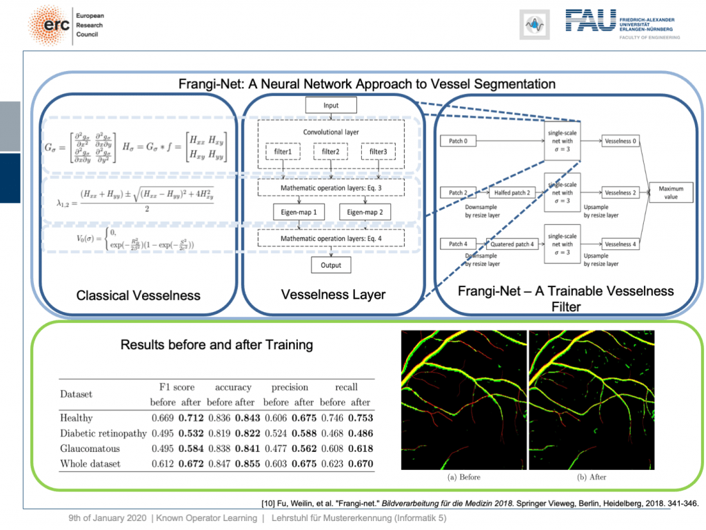
Very well, there are also other things that we can use as a kind of prior knowledge. Here is a work where we essentially took a heuristic method, the so-called vesselness filter that has been proposed by Frangi. You can show that the processing that it does is essentially convolutions. There’s an eigenvalue computation. But if you look at the eigenvalue computation, you can see that this central equation here. It can also be expressed as a layer and this way we can map the entire computations of the Frangi filter into a specialized kind of layer. This can then be trained in a multiscale approach and gives you a trainable version of the Frangi filter. Now, if you do so, you can produce vessel segmentations and they are essentially inspired by the Frangi filter but because they are trainable they produce much better results.
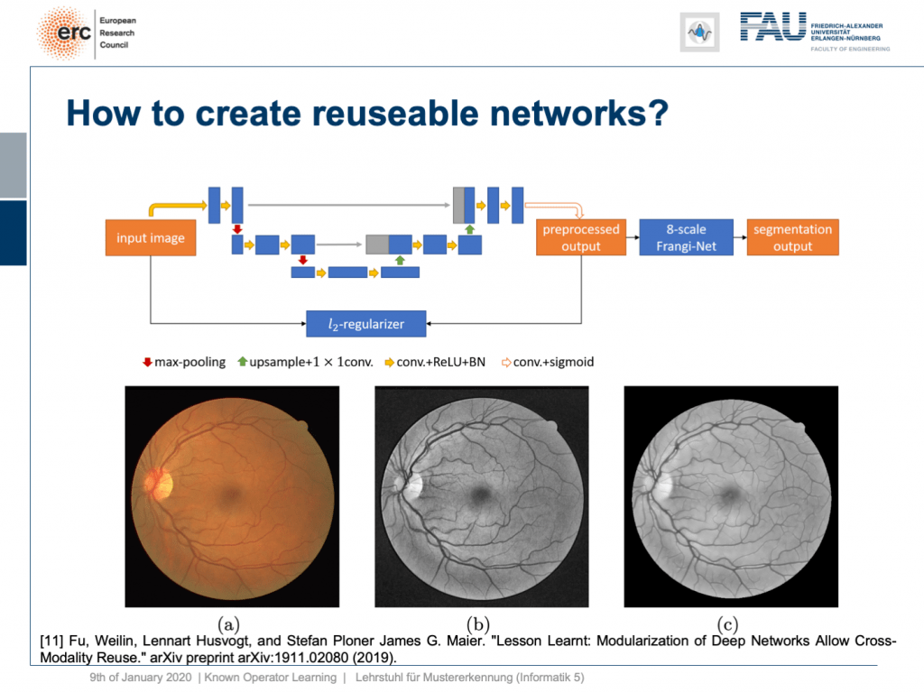
This is kind of interesting, but you very quickly realize that one reason why the Frangi filter fails is inadequate pre-processing. So, we can also combine this with a kind of pre-processing network. Here, the idea then is that you take let’s say a U-net or a guided filter network. Also, the guided filter or by the way the joint bilateral filter can be mapped into neural network layers. You can include them here and you design a special loss. This special loss is not just optimizing the segmentation output, but you combine it with some kind of autoencoder loss here. So in this layer, you want to have a pre-processed image that is still similar to the input, but with properties such that the vessel segmentation using an 8 scale Frankie filter is much better. So, we can put this into our network and train it. As a result, we get vessel detection and this vessel detection is on par with a U-net. Now, the U-Net is essentially a black box method, but here we can say “Okay, we have a kind of pre-processing net.” By the way, using a guided filter, it works really well. So, it doesn’t have to be a U-net. This is kind of a neural network debugging approach. You can show that we can now module by module replace parts of our U-net. In the last version, we don’t have U-nets at all anymore, but we have a guided filter network here and the Frangi filter. This has essentially the same performance as the U-net. So, this way we are able to modularize our networks. Why would you want to create modules? Well, the reason is modules are reusable. So here, you see the output on eye imaging data of ophthalmic data. This is a typical fundus image. So it’s an RGB image of the eye background. It shows the blind spot where the vessels all penetrate the retina. The fovea is where you have essentially the best resolution on your retina. Now, typically if you want to analyze those images, you would just take the green color Channel because it’s the channel of the highest contrast. The result of our pre-processing network can be shown here. So, we get significant noise reduction, but at the same time, we also get this emphasis on vessels. So, it kind of improves how the vessels are displayed and also fine vessels are preserved.
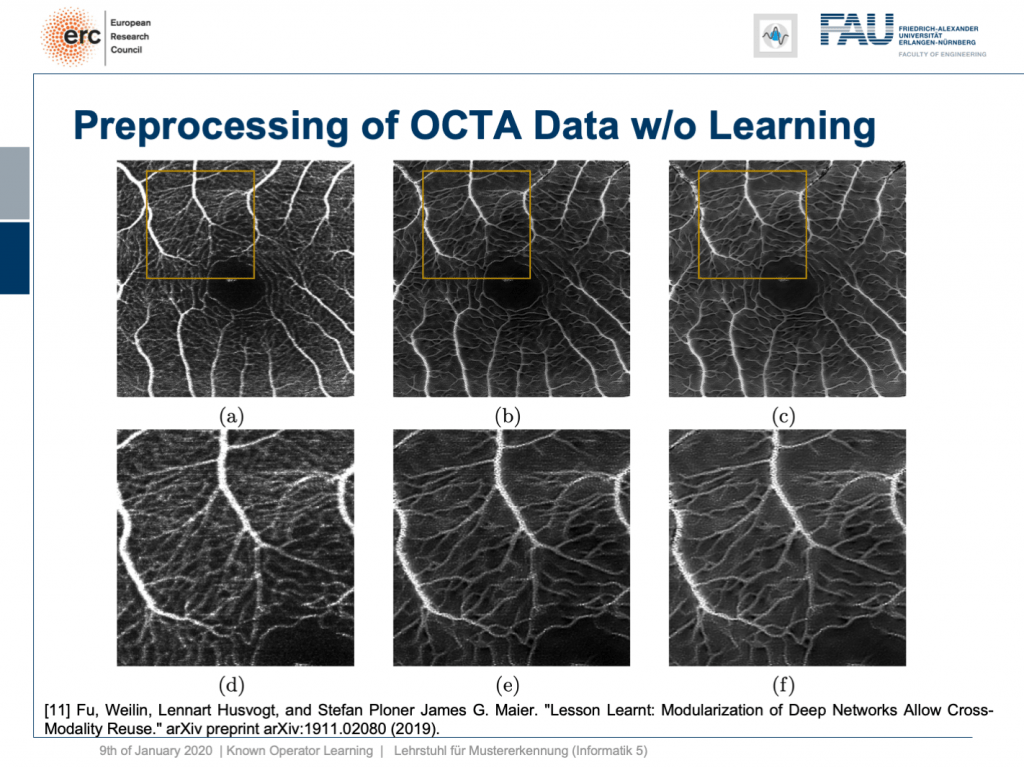
Okay, this is nice, but it only works on fundus data, right? No, our modularization shows that if we take this kind of modeling, we are able to transfer the filter to a completely different modality. This is now optical cohere tomography angiography (OCTA), a specialist modality in order to extract contrast-free vessel images of the eye background. You can now demonstrate that our pre-processing filter can be applied to these data without any additional need for fine-tuning, learning, or whatnot. You take this filter and apply it to the en-face images that, of course, show similar anatomy. But you don’t need any training on OCTA data at all. This is the OCTA input image on the left. This is the output of our filter, in the center, and this is a 50% blend of the two, on the right. Here, we have the magnified areas and you can see very nicely that what is appearing like noise is actually reformed into vessels in the output of our filter. Now, these are qualitative results. By the way, until now we finally also have quantitative results and we are actually quite happy that our pre-processing network is really able to produce the vessels at the right locations. So, this is a very interesting result and this shows us that we kind of can modularize networks and make them reusable without having to train them. So, we can now probably generate blocks that can be reassembled to new networks without additional adjustment and fine-tuning. This is actually pretty cool.
Well, this essentially leads us back to our classical pattern recognition pipeline. You remember, we looked at that in the very beginning. We have the sensor, the pre-processing, the features, and the classification. The classical role of neural networks was just classifying and you had all these feature engineering on the path here. We said that’s much better to do deep learning because then we do everything end-to-end and we can optimize all on the way. Now, if we look at this graph then we can also think about whether we actually need something like neural network design patterns. One design pattern is of course the end-to-end learning, but you may also want to include these autoencoder pre-processing losses in order to get the maximum out of your signals. On the one hand, you want to make sure that you have an interpretable module here that still remains in the image domain. On the other hand, you want to have good features and another thing that we learned about in this class is multi-task learning. So, multi-task learning associates the same latent space with different problems with different classification results. This way by implementing a multi-task loss, we make sure that we get very general features and features that will be applicable to a wide range of different tasks. So, essentially we can see that by appropriate construction of our loss functions, we’re actually back to our classical pattern recognition pipeline. It’s not the same pattern recognition pipeline that we had in a classical sense because everything is end-to-end and differentiable. So, you could argue that what we’re going towards right now is CNNs, ResNets, global pooling, differentiable rendering even are kinds of known operations that are embedded into those networks. We then essentially get modules that can be recombined and we probably end up in differentiable algorithms. This is the path that we’re going: Differentiable, adjustable algorithms that can be fine-tuned using only a little bit of data.
I wanted to show to you this concept because I think known operator learning is pretty cool. It also means that you don’t have to throw away all of the classical theory that you already learned about: Fourier transforms and all the clever ways of how you can process a signal. They still are very useful and they can be embedded into your networks, not just using regularization and losses. We’ve already seen when we talked about this bias-variance tradeoff, this is essentially one way how you can reduce variance and bias at the same time: You incorporate prior knowledge on the problem. So, this is pretty cool. Then, you can create algorithms, learn the weights, you reduce the number of parameters. Now, we have a nice theory that also shows us that what we are doing here is sound and virtually all of the state-of-the-art methods can be integrated. There are very few operations where you cannot find a subgradient approximation. If you don’t find a subgradient approximation, there are probably also other ways around it, such that you can still work with it. This makes methods very efficient, interpretable, and you can also work with modules. So, that’s pretty cool, isn’t it?
Well, this is our last video. So, I also want to thank you for this exciting semester. This is the first time that I am entirely teaching this class in a video format. So far, what I heard, the feedback was generally very positive. So, thank you very much for providing feedback on the way. This is also very crucial and you can see that we improved on the lecture on various occasions in terms of hardware and also in what to include, and so on. Thank you very much for this. I had a lot of fun with this and I think a lot of things I will also keep on doing in the future. So, I think these video lectures are a pretty cool way, in particular, if you’re teaching a large class. In the non-corona case, this class would have an audience of 300 people and I think, if we use things like these recordings, we can also get a very personal way of communicating. I can also use the time that I don’t spend in the lecture hall for setting up things like question and answer sessions. So, this is pretty cool. The other thing that’s cool is we can even do lecture notes. Many of you have been complaining, the class doesn’t have lecture notes and I said “Look, we make this class up-to-date. We include the newest and coolest topics. It’s very hard to produce lecture notes.” But actually, deep learning helps us to produce lecture notes because have video recordings. We can use speech recognition on the audio track and produce lecture notes. So you see that I already started doing this and if you go back to the old recordings, you can see that I already put in links to the full transcript. They’re published as blog posts and you can also access them. By the way, like the videos are the blog posts and everything that you see here licensed using Creative Commons BY 4.0 which means you are free to reuse any part of this and redistribute and share it. So generally, I think this field of machine learning and in particular, deep learning methods we’re going at a rapid pace right now. We are still going ahead. So, I don’t see that these things and developments will stop very soon and there’s still very much excitement in the field. I’m also very excited that I can show the newest things to you in lectures like this one. So, I think there are still exciting new breakthroughs to come and this means that we will adjust this lecture also in the future, produce new lecture videos in order to be able to incorporate the newest latest and greatest methods.
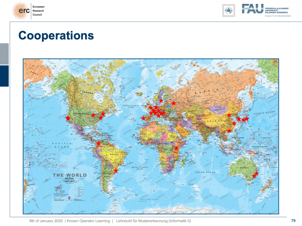
By the way, the stuff that I’ve been showing you in this lecture is of course not just by our group. We incorporated many, many different results by other groups worldwide and of course with results that we produced in Erlangen, we do not alone, but we are working in a large network of international partners. I think this is the way how science needs to be conducted, also now and in the future. I have some additional references. Okay. So, that’s it for this semester. Thank you very much for listening to all of these videos. I hope you had quite some fun with them. Well, let’s see I’m pretty sure I’ll teach a class next semester again. So, if you like this one, you may want to join one of our other classes in the future. Thank you very much and goodbye!
If you liked this post, you can find more essays here, more educational material on Machine Learning here, or have a look at our Deep LearningLecture. I would also appreciate a follow on YouTube, Twitter, Facebook, or LinkedIn in case you want to be informed about more essays, videos, and research in the future. This article is released under the Creative Commons 4.0 Attribution License and can be reprinted and modified if referenced. If you are interested in generating transcripts from video lectures try AutoBlog.
Thanks
Many thanks to Weilin Fu, Florin Ghesu, Yixing Huang Christopher Syben, Marc Aubreville, and Tobias Würfl for their support in creating these slides.
References
[1] Florin Ghesu et al. Robust Multi-Scale Anatomical Landmark Detection in Incomplete 3D-CT Data. Medical Image Computing and Computer-Assisted Intervention MICCAI 2017 (MICCAI), Quebec, Canada, pp. 194-202, 2017 – MICCAI Young Researcher Award
[2] Florin Ghesu et al. Multi-Scale Deep Reinforcement Learning for Real-Time 3D-Landmark Detection in CT Scans. IEEE Transactions on Pattern Analysis and Machine Intelligence. ePub ahead of print. 2018
[3] Bastian Bier et al. X-ray-transform Invariant Anatomical Landmark Detection for Pelvic Trauma Surgery. MICCAI 2018 – MICCAI Young Researcher Award
[4] Yixing Huang et al. Some Investigations on Robustness of Deep Learning in Limited Angle Tomography. MICCAI 2018.
[5] Andreas Maier et al. Precision Learning: Towards use of known operators in neural networks. ICPR 2018.
[6] Tobias Würfl, Florin Ghesu, Vincent Christlein, Andreas Maier. Deep Learning Computed Tomography. MICCAI 2016.
[7] Hammernik, Kerstin, et al. “A deep learning architecture for limited-angle computed tomography reconstruction.” Bildverarbeitung für die Medizin 2017. Springer Vieweg, Berlin, Heidelberg, 2017. 92-97.
[8] Aubreville, Marc, et al. “Deep Denoising for Hearing Aid Applications.” 2018 16th International Workshop on Acoustic Signal Enhancement (IWAENC). IEEE, 2018.
[9] Christopher Syben, Bernhard Stimpel, Jonathan Lommen, Tobias Würfl, Arnd Dörfler, Andreas Maier. Deriving Neural Network Architectures using Precision Learning: Parallel-to-fan beam Conversion. GCPR 2018. https://arxiv.org/abs/1807.03057
[10] Fu, Weilin, et al. “Frangi-net.” Bildverarbeitung für die Medizin 2018. Springer Vieweg, Berlin, Heidelberg, 2018. 341-346.
[11] Fu, Weilin, Lennart Husvogt, and Stefan Ploner James G. Maier. “Lesson Learnt: Modularization of Deep Networks Allow Cross-Modality Reuse.” arXiv preprint arXiv:1911.02080 (2019).