Lecture Notes in Deep Learning: Introduction – Part 3

Limitations of Deep Learning and Future Directions

These are the lecture notes for FAU’s YouTube Lecture “Deep Learning“. This is a full transcript of the lecture video & matching slides. We hope, you enjoy this as much as the videos. Of course, this transcript was created with deep learning techniques largely automatically and only minor manual modifications were performed. If you spot mistakes, please let us know!

Thanks for tuning in to the next video of deep learning. So, what I want to show you in this video are a couple of limitations of deep learning. So, you may wonder are there any limitations? Are we done yet? Aren’t we learning something here that will solve all of the problems?

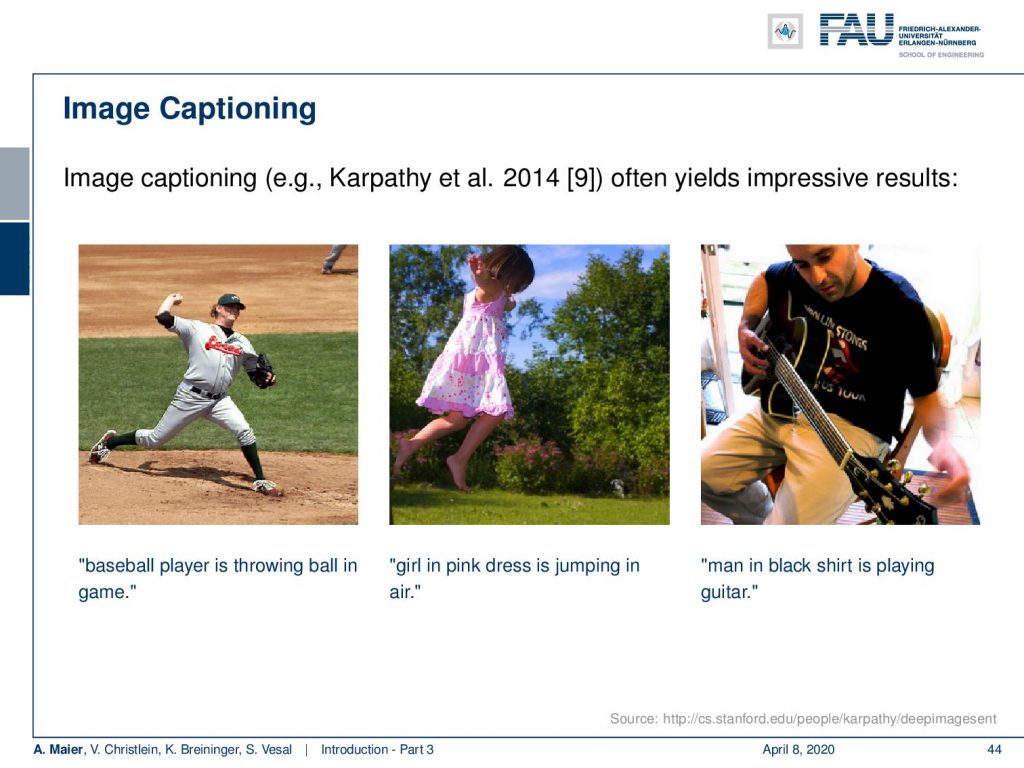
Well of course there are some limitations. For example tasks like image captioning yield impressive results. You can see that the networks are able to identify the baseball player, the girl in a pink dress jumping in the air, or even people playing the guitar.

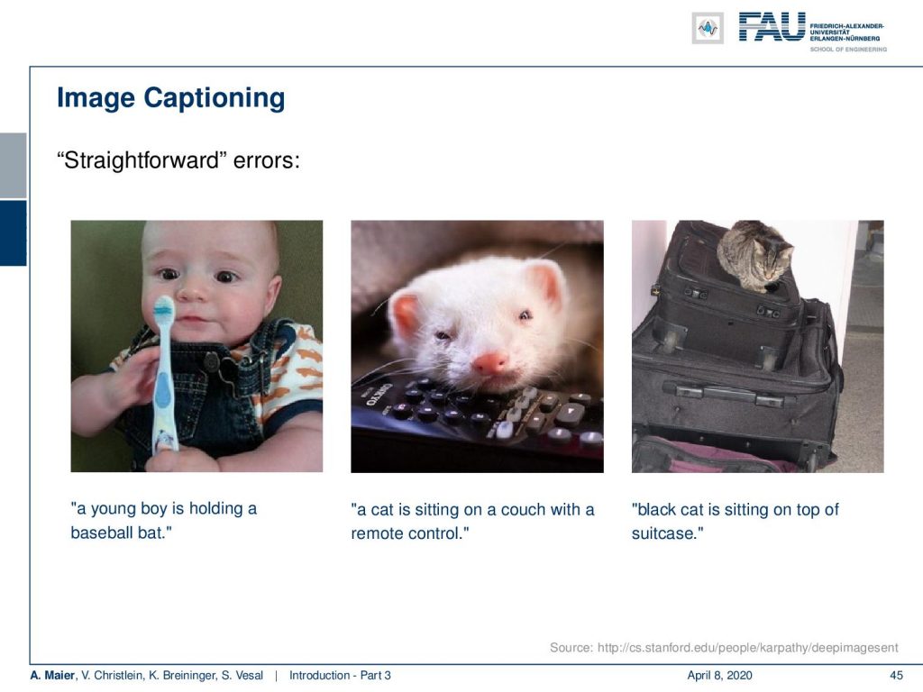
So let’s look at some errors. Here on the left, you can see, this is clearly not a baseball bat. Also, this isn’t a cat in the center image and they are also slight errors like the one on the right-hand side: The cat on top of the suitcases isn’t black.

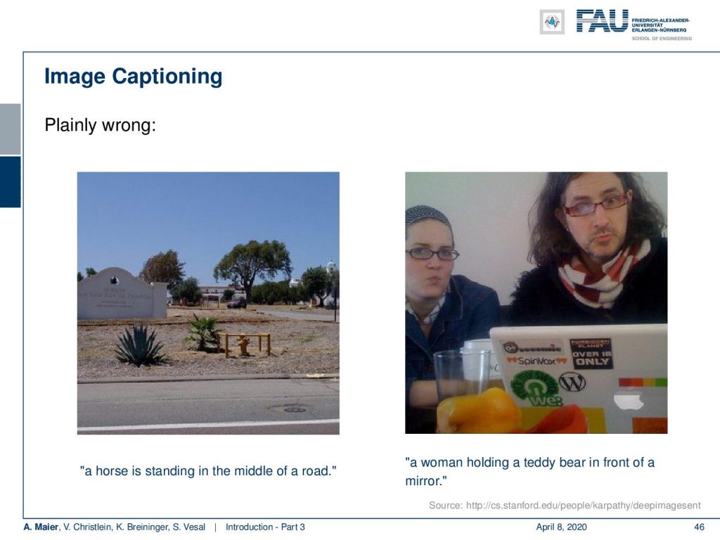
Sometimes they’re even plain errors like here in the left image: There, I don’t see a horse in the middle of the road and also on the right image there is no woman holding a teddy bear in front of a mirror.

So, the reason for this is of course there’s a couple of challenges and one major challenge is training data. Deep learning applications require huge manually annotated data sets and these are hard to obtain. Annotation is time-consuming and expensive and often ambiguous. So, as you’ve seen already in the image net challenge, sometimes it’s not clear which label to assign, and obviously you would have to assign a distribution of labels. Also, we see that even in the human annotations, there are typical errors. What you have to do in order to get a really good representation of the labels, you actually have to ask two or even more experts to do the entire labeling process. Then, you can find out the instances where you have a very sharp distribution of labels. These are typical prototypes and broad distributions of labels are images where people are not sure. If we have such problems, then we typically get a significant drop in performance. So the question is how far can we get simulations for example to expand training data.

Of course, there are also challenges with trust and reliability. So, verification is mandatory for high-risk applications, and regulators can be very strict about those. They really want to understand what’s happening in those high-risk systems. End-to-end learning essentially prohibits to identify how the individual parts work. So, it’s very hard for regulators to tell what part does what and why the system actually works. We must admit at this point that this is largely unsolved to a large degree. It’s difficult to tell which part of the network is doing what. Modular approaches that are based on classical algorithms may be one approach to solve these problems in the future.

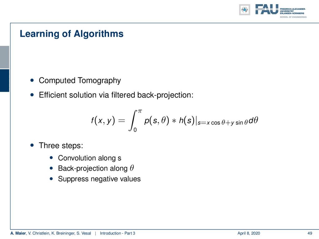
This brings us to the future directions and something that we like to do here in Erlangen is learning algorithms. So for example, you can look at the classical computer tomography which is expressed in the filtered back-projection formula. You have to filter along the projection direction and then a summation over the angle in order to produce a final image. So this convolution and back-projection then can actually be expressed in terms of linear operators. As such, they are essentially matrix multiplications.

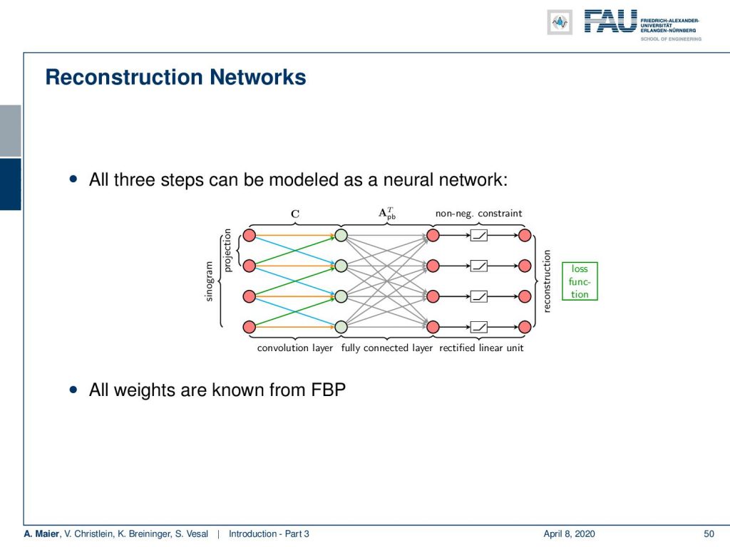
Now, those matrix multiplications can be implemented as a neural network and you essentially then have an algorithm or a network design that can be trained for specific purposes.

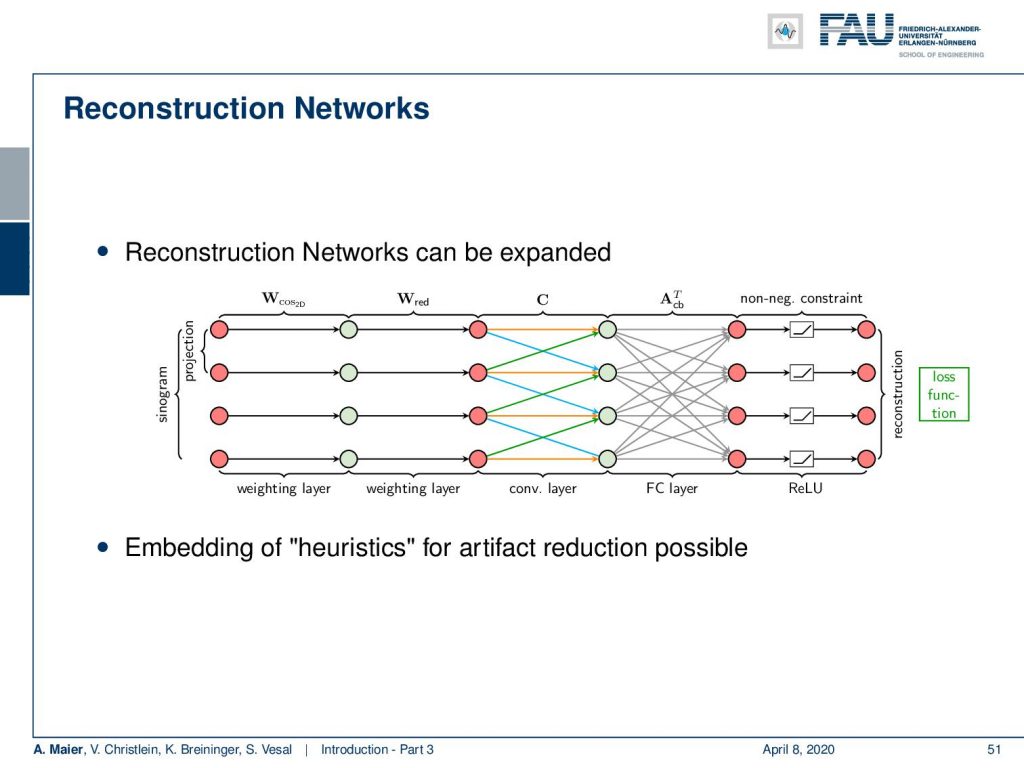
So here, we extend this approach in order to apply it to fan-beam projection data. This is a slight modification of the algorithm. There are cases that cannot be solved like the limited angle situation.

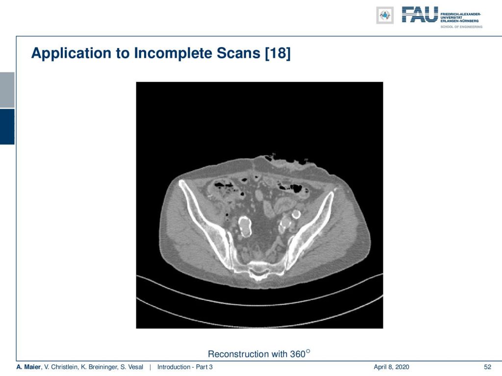
In this image, you see a full scan and this produces a reasonable CT image. However, if you’re missing only twenty degrees of rotation you already see severe artifacts:

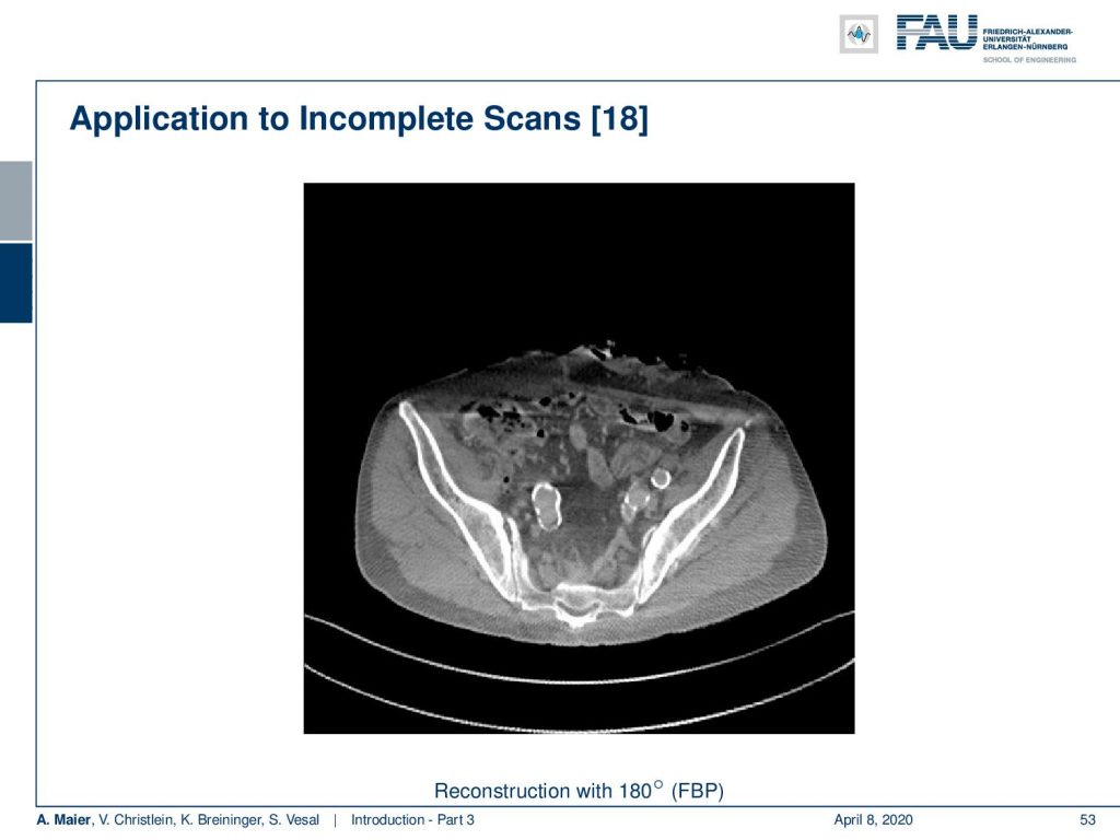
Now, if you take the idea of converting your reconstruction algorithm into a neural network and retrain it on some training data. Here it’s only 15 images and you can see that even on unseen data, we are able to recover most of the lost information:

Now, if you look at the top part of this image you can see that there is a reduction of mass. We show line plots following the red line in the left image on the right-hand side:

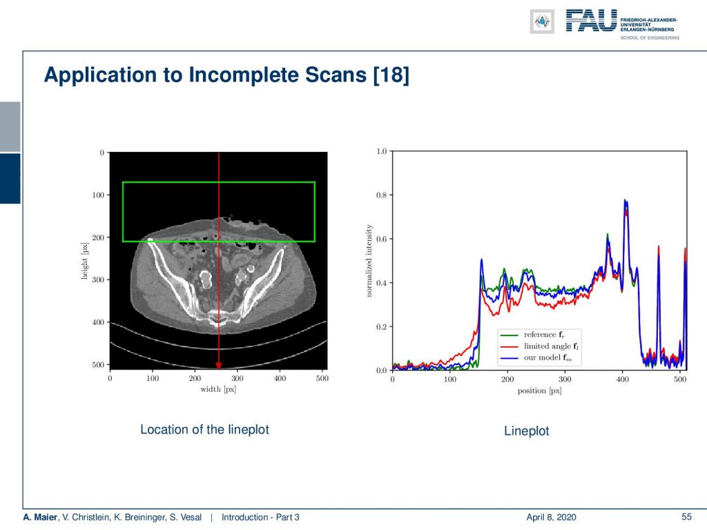
Now here in green, you can see the reference image that is largely unaffected. As soon as you introduce the angle limitation, you end up with the red curve which shows these artifacts in the top part of the image. Now, if you further go ahead and take our deep learning method, you end up with the blue curve which largely reduces problems that have been introduced by the angular and limitation. Now, the fun part about this is because our algorithm has been inspired by a traditional CT reconstruction algorithm, all of those layers have interpretations: They are linked to a specific function. What do you typically do for such a short scan, is that you weight down rays that have been measured twice, such that the opposing rays exactly sum to one.

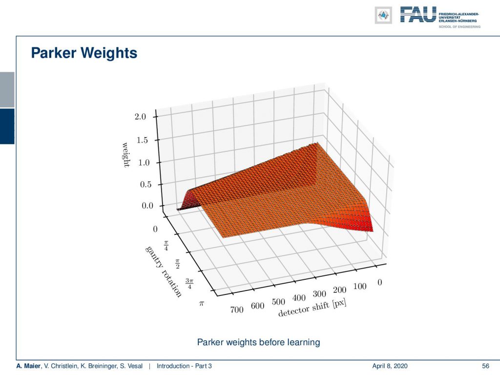
You can see that here the Parker Weights in this figure. Now, if we train our algorithm, the main changes are the Parker weights. What happens is that we can see an increase of weight in particular in rays that run through the area that has the angular limitation after training:

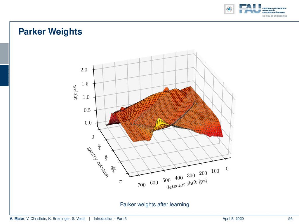
So, the network learns to use the information from a slightly different direction in those rays that have not been measured. You can even go ahead and then combine this reconstruction method with additional de-streaking and denoising steps and as we will show towards the end of this lecture. As a result, we can dramatically improve also in the low contrast information.

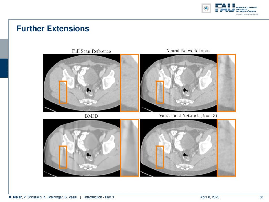
Here, you see an image of the full scan reference on the top left, the neural network output on the top right that still has significant streaks, and on the bottom right, you see a streak reduction network. It is able to really reduce those streaks that have been caused by the angular limitation. Compared to just a denoising approach on the bottom left, you can see that those streaks would be diminished but they still would be present. Only such a trained method that understands what the problem is, is actually able to reduce those artifacts efficiently.

So next time in deep learning, we want to look at basic pattern recognition and machine learning. Which basic rules are there and how this is in relation to deep learning? Then, we want to go ahead and talk about the perceptron which is the basic unit of a neural network. From those perceptrons, you can build those really deep networks that we have been featuring in this and previous videos. So, I hope you like this video and it would be really great if you tune in next time. Thank you!

If you liked this post, you can find more essays here, more educational material on Machine Learning here, or have a look at our Deep Learning Lecture. I would also appreciate a clap or a follow on YouTube, Twitter, Facebook, or LinkedIn in case you want to be informed about more essays, videos, and research in the future. This article is released under the Creative Commons 4.0 Attribution License and can be reprinted and modified if referenced.

References

[1] David Silver, Julian Schrittwieser, Karen Simonyan, et al. “Mastering the game of go without human knowledge”. In: Nature 550.7676 (2017), p. 354.
[2] David Silver, Thomas Hubert, Julian Schrittwieser, et al. “Mastering Chess and Shogi by Self-Play with a General Reinforcement Learning Algorithm”. In: arXiv preprint arXiv:1712.01815 (2017).
[3] M. Aubreville, M. Krappmann, C. Bertram, et al. “A Guided Spatial Transformer Network for Histology Cell Differentiation”. In: ArXiv e-prints (July 2017). arXiv: 1707.08525 [cs.CV].
[4] David Bernecker, Christian Riess, Elli Angelopoulou, et al. “Continuous short-term irradiance forecasts using sky images”. In: Solar Energy 110 (2014), pp. 303–315.
[5] Patrick Ferdinand Christ, Mohamed Ezzeldin A Elshaer, Florian Ettlinger, et al. “Automatic liver and lesion segmentation in CT using cascaded fully convolutional neural networks and 3D conditional random fields”. In: International Conference on Medical Image Computing and Computer-Assisted Springer. 2016, pp. 415–423.
[6] Vincent Christlein, David Bernecker, Florian Hönig, et al. “Writer Identification Using GMM Supervectors and Exemplar-SVMs”. In: Pattern Recognition 63 (2017), pp. 258–267.
[7] Florin Cristian Ghesu, Bogdan Georgescu, Tommaso Mansi, et al. “An Artificial Agent for Anatomical Landmark Detection in Medical Images”. In: Medical Image Computing and Computer-Assisted Intervention – MICCAI 2016. Athens, 2016, pp. 229–237.
[8] Jia Deng, Wei Dong, Richard Socher, et al. “Imagenet: A large-scale hierarchical image database”. In: Computer Vision and Pattern Recognition, 2009. CVPR 2009. IEEE Conference IEEE. 2009, pp. 248–255.
[9] A. Karpathy and L. Fei-Fei. “Deep Visual-Semantic Alignments for Generating Image Descriptions”. In: ArXiv e-prints (Dec. 2014). arXiv: 1412.2306 [cs.CV].
[10] Alex Krizhevsky, Ilya Sutskever, and Geoffrey E Hinton. “ImageNet Classification with Deep Convolutional Neural Networks”. In: Advances in Neural Information Processing Systems 25. Curran Associates, Inc., 2012, pp. 1097–1105.
[11] Joseph Redmon, Santosh Kumar Divvala, Ross B. Girshick, et al. “You Only Look Once: Unified, Real-Time Object Detection”. In: CoRR abs/1506.02640 (2015).
[12] J. Redmon and A. Farhadi. “YOLO9000: Better, Faster, Stronger”. In: ArXiv e-prints (Dec. 2016). arXiv: 1612.08242 [cs.CV].
[13] Joseph Redmon and Ali Farhadi. “YOLOv3: An Incremental Improvement”. In: arXiv (2018).
[14] Frank Rosenblatt. The Perceptron–a perceiving and recognizing automaton. 85-460-1. Cornell Aeronautical Laboratory, 1957.
[15] Olga Russakovsky, Jia Deng, Hao Su, et al. “ImageNet Large Scale Visual Recognition Challenge”. In: International Journal of Computer Vision 115.3 (2015), pp. 211–252.
[16] David Silver, Aja Huang, Chris J. Maddison, et al. “Mastering the game of Go with deep neural networks and tree search”. In: Nature 529.7587 (Jan. 2016), pp. 484–489.
[17] S. E. Wei, V. Ramakrishna, T. Kanade, et al. “Convolutional Pose Machines”. In: CVPR. 2016, pp. 4724–4732.
[18] Tobias Würfl, Florin C Ghesu, Vincent Christlein, et al. “Deep learning computed tomography”. In: International Conference on Medical Image Computing and Computer-Assisted Springer International Publishing. 2016, pp. 432–440.

Category: Lecture Notes in Deep Learning