
Highlights at FAU
These are the lecture notes for FAU’s YouTube Lecture “Deep Learning“. This is a full transcript of the lecture video & matching slides. We hope, you enjoy this as much as the videos. Of course, this transcript was created with deep learning techniques largely automatically and only minor manual modifications were performed. If you spot mistakes, please let us know!
So, thank you very much for tuning in again and welcome to our second part of the deep learning lecture and in particular the introduction. So, in the second part of the introduction, I want to show you some research that we are doing here in the pattern recognition lab, here at FAU Germany.
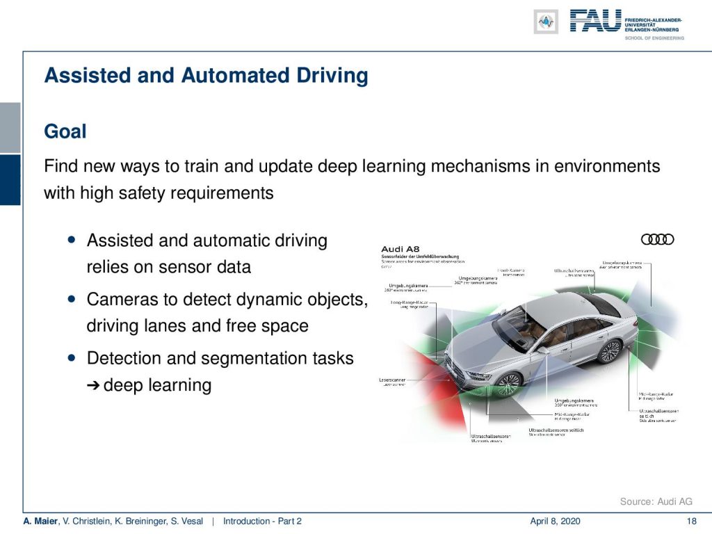
One first example that I want to highlight is a cooperation with Audi and here we are working with assisted and automated driving. We are working on smart sensors in the car. You can see that the Audi A8 today is essentially a huge sensor system that has cameras and different sensors attached. Data is processed in real-time in order to figure out things about the environment. It has functionalities like parking assistance. There are also functionalities to support you during driving and traffic jams and this is all done using sensor systems. So of course, there’s a lot of detection and segmentation tasks involved.
What you can see here is an example, where we show some output of what is recorded by the car. This is a frontal view, where we are actually looking around the surroundings and have to detect cars. You also have to detect – here shown in green – the free space where you can actually drive to and all of this has to be detected and many of these things are done with deep learning. Today, of course, there’s a huge challenge because we need to test the algorithms. Often this is done in simulated environments and then a lot of data is produced in order to make them reliable. But in the very end, this has to run on the road which means that you have to consider different periods of the year and different daylight conditions. This makes it all extremely hard. What you’ve seen in research is that many of the detection results are working with nice day scenes and the sun is shining. Everything is nice, so the algorithms work really well.
But the true challenge is actually to go towards rainy weather conditions, night, winter, snow, and you still want to be able to detect, of course, not just cars but traffic signs and landmarks. Then you analyze the scenes around you such that you have a reliable prediction towards your autonomous driver system.
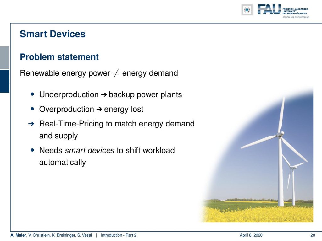
We also look into smart devices and of course, some very interesting topic here is renewable energy and power. One problem that we typically face is under production, when there’s not enough wind blowing or when not enough sun is shining. Then, you have to fire up backup power plants and, of course, you don’t want to do overproduction because that would produce energy that cannot be stored very well. The storing of energy is not very efficient right now. There are some ideas to tackle this like real-time prices but what you need are smart devices that can recognize and predict how much power is going to be produced in the near future.
So, let’s look at an example of smart devices. So let’s say, you have a fridge or a washing machine and you can program them in a way that they are flexible at the point in time when they consume the energy. You can start the washing also maybe overnight or in one hour when the price is lower. So, if you had smart devices that could predict the current prices, then you would be able to essentially balance the nodes of the energy system and at the same time remove the peak conditions. Let’s say there’s a lot of wind blowing. Then, it would make sense that a lot of people cool down the refrigerator or wash their dishes or their clothes. So this can be done of course with recurrent neural networks and then you predict how much power will be produced and use it on the client-side to level the power production.
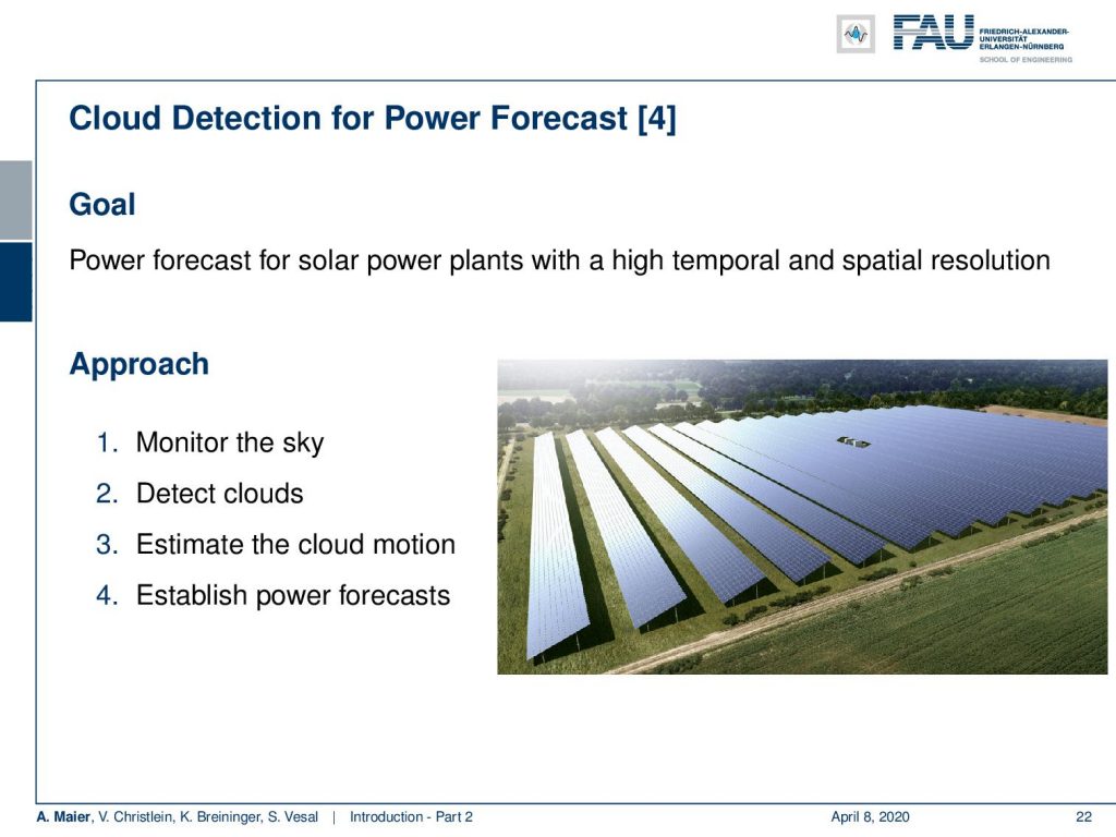
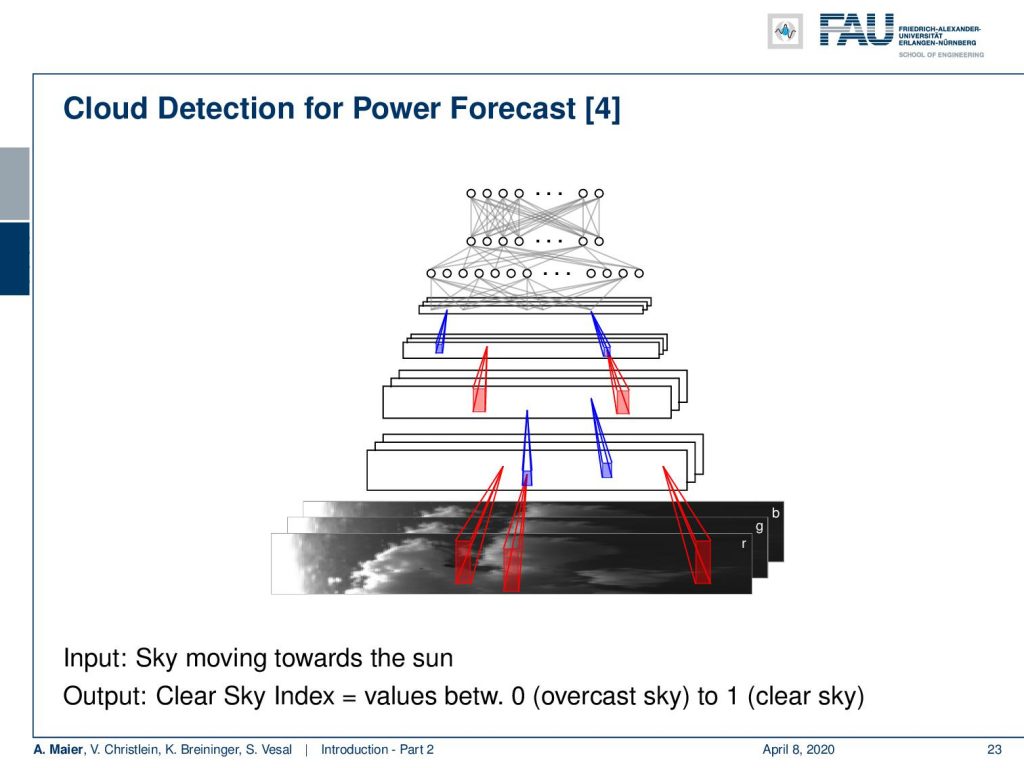
This example here shows a solar power plant. They were interested in predicting the short-term power production in order to inform other devices or to fire up backup power plants. The crucial timeframe here is approximately 10 minutes. So, the idea here was to monitor the sky, to detect the clouds, to estimate the cloud motion, and then directly predict from the current sky image, how much power will be produced within the next 10 minutes. So, let’s say there’s a cloud that is likely to be covering the Sun really soon. Then, you want to fire up generators or inform devices not to consume so much energy. Now clouds are really difficult to describe in terms of an algorithm but what we are doing here is that we are using a deep network to try to learn the representation. These deep learning features are predictive for power production and we actually managed to produce reliable predictions for approximately 10 minutes. With traditional pattern recognition techniques, we could only do predictions of approximately 5 minutes.
Another very exciting topic that I want to demonstrate today, is writer recognition. Now here, the task is that you have a piece of writing and you want to find out who wrote actually this text. So, we are not recognizing what was written but who has written the text. The idea here is again to train a deep network and this deep network is then learning abstract features that describe how a person is writing. So it’s only looking at small patches around the letters and these small patches around the letters are used in order to predict who has actually written the text.

A colleague of mine just showed in a very nice submission that he just submitted to an international conference that he is also able to generate handwriting that is distinctive for a particular person. Like many methods, you can see that these deep learning approaches can of course be used for very good purposes like identifying what a person wrote this in historical texts. But then you can also use very similar methods to produce fakes and to spread misinformation. So you can see that in a lot of technology and of course this is a reason why ethics are very important also in the field of deep learning.
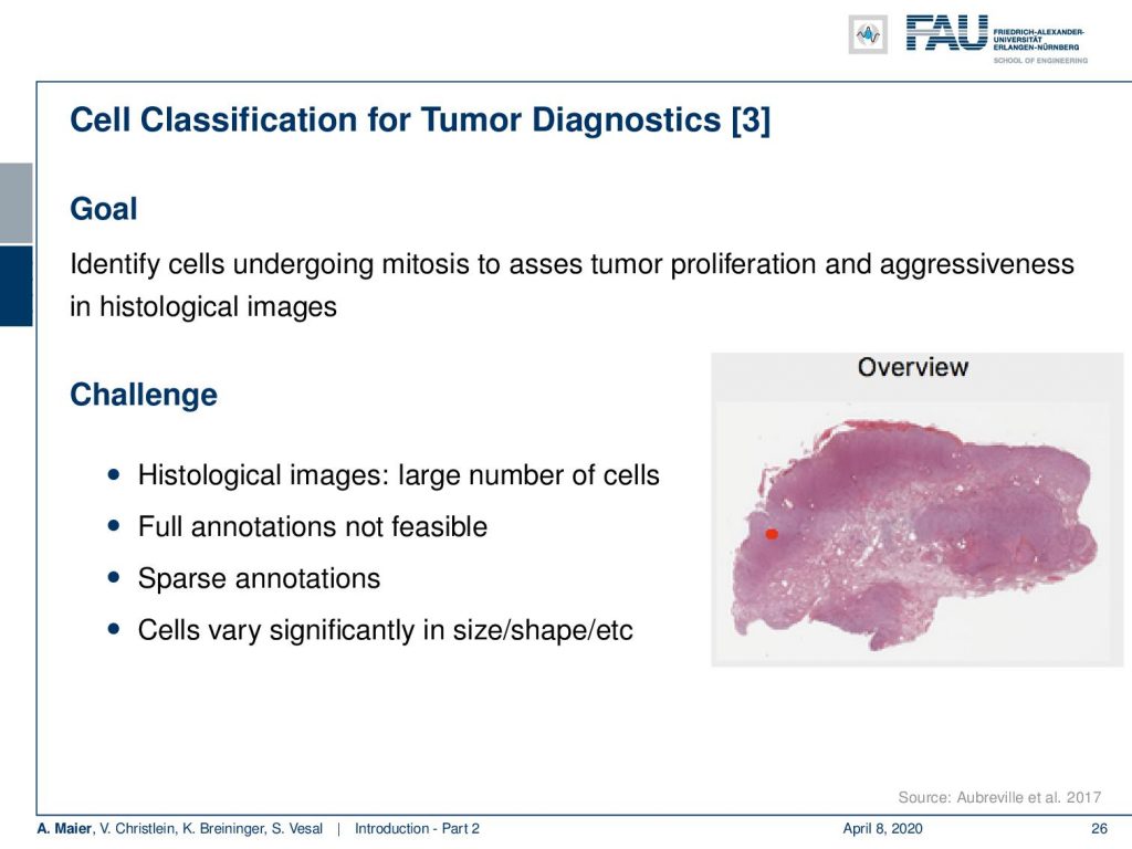
Most of the work that we are doing is actually concerning medical applications. A really cool application of deep learning is where you want to screen a really large part of data. So a colleague of mine just started looking into whole slide images. This is for tumor Diagnostics, for example where you’re interested to figure out how aggressive a cancer is. You can figure out, how aggressive a cancer is if you look at the number of cell divisions that are going on at a certain point in time. So, you are actually interested in not just finding out the cancer cells, but you want to find how often these cancer cells actually undergo mitosis, i.e. cell division. The number of detected mitoses is indicative of how aggressive this particular cancer is. Now, these whole slide images are very big and you don’t want to look at every cell individually. What you can do, is that you can train a deep network to look at all of the cells and then do the analysis for the entire whole slide in clinical routine. Currently, people are not looking at the entire slide image. They are looking at high power fields, like the small part that you can see here on this image.
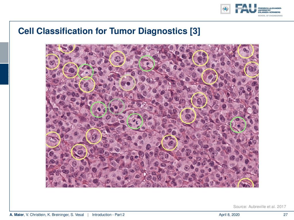
This is a high power field. In clinical routine, they count the mitosis within this field of view. So of course, they just don’t do it on a single high power field. They typically look at ten high power fields to assess the aggressiveness of cancer. With the deep learning method you could process all of the slide.
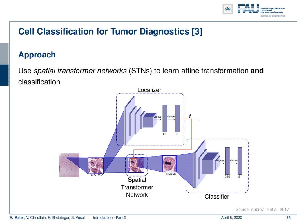
So this is how such a deep learning approach would look like. You have some part in the network that localizes the cells and then a different part of the network that is then classifying the cell, whether it’s a mitosis, a regular cell, or a cancer cell.
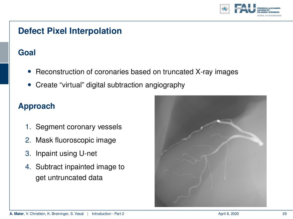
Very interesting things can also be done with defect pixel interpolation. So here, we see a small scene where we show the coronary arteries of the heart. Typically those coronary arteries are not stationary. They are moving and because they are moving it’s very hard to see and analyze them. So what is typically done to create clear images of the coronary arteries is you inject contrast agent and the reason why you can actually see the coronary arteries in this image is because they are right now filled with iodine-based contrast agent. Otherwise, because blood is very close to water in terms of X-ray absorption, you wouldn’t be able to see anything.
A very common technique to visualize the arteries is to take two images: one with contrast agent and one without. Now, if you subtract the two you would only see the contrast agent. In a cardiac intervention, this is very difficult because the heart is moving all the time and the patient is breathing. Therefore it is very hard to apply techniques like digital subtraction angiography.
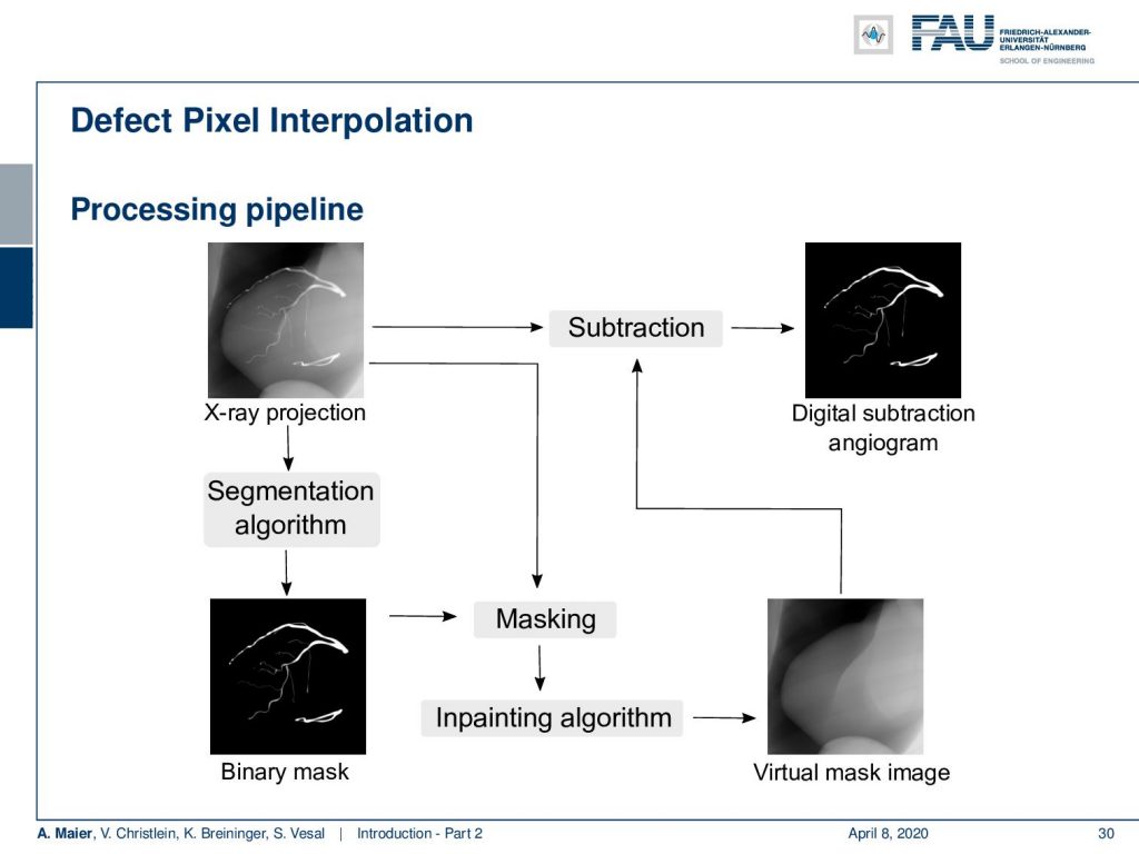
Here we propose to segment the detected vessels. So, we use a deep learning framework that is actually segmenting the vessels. Once we have the vessel segmentation, we use this as a mask. Then, we use a deep learning method to predict the pixels of the mask if there were no contrast agent. This will make those pixels disappear from the image. Now, you can take this virtual non-contrast image and subtracted from the original projection and you get a digital subtraction angiogram. This technique also works for images in motion. So this is something that could not be done without techniques of deep learning. The actual implementation for the interpolation is done by a U-Net. This is something that you will hear in the latter part of this lecture when we are talking about image segmentation where it’s typically used. The U-Net is a general image to image transformer. You can also use it to produce contrast free images.
Another important part that is often done in whole-body images is that you want to localize different organs. My colleague Florin Ghesu developed a smart method in order to figure out where the different organs are. So, the idea is to process the image in a very similar way as you would do as a radiologist: You start off by looking at a small part of the image and then you try to predict where you have to go to find that specific organ of interest. Of course, doing this on a single resolution level is insufficient. Thus, you’re then also refining the search on smaller resolution levels in order to get a very precise prediction of the organ centroid. This kind of prediction is very fast because you only look at a fraction of the volume. So you can do 200 anatomical landmarks in approximately two seconds. The other very interesting part is that you produce a path that can also then be interpreted. Even in cases where the specific landmark is not present in the volume this approach does not fail. So, let’s say you look for the hipbone in a volume that doesn’t even show the hip. Then you will see that the virtual agent tries to leave the volume and it will not predict a false position. Instead, it will show you that the hipbone would be much lower and you have to leave the volume at this place.
Landmark detection can also be used in projection images as demonstrated by my colleague Bastian Bier. He developed a very interesting method where you are using the 3-D position of landmarks. With the 3-D position, you create virtual projections of the landmark and train a projection image-based classifier. With the projection image-based classifier, you can detect the landmark in arbitrary views of the specific anatomy under interest. So here, we show an example for the hipbone and you can see that if we forward project it and try to detect the landmarks, it’s actually a pretty hard task. With the method that Bastion has devised, we are able to track the entire hip bone and to find the specific landmarks on the hip bone directly from the projection views. So the idea here is that you use a convolutional pose machine. Here we essentially process each landmark individually and then you inform the different landmarks that have been detected in the first part about the respective other landmarks’ positions. Then, you process again and again until you have a final landmark position.
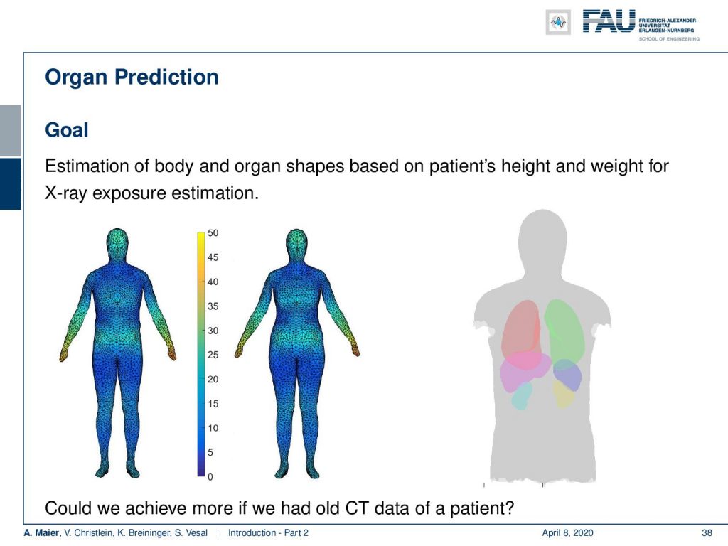
My colleague Xia Zhong has been working on prediction of organ positions and what he has been doing is he is essentially using a 3-D camera to detect the surface of the patient. Then, he wants to predict where the organs are actually located inside the body. Now, this is very interesting because we can use the information to predict how much radiation dose will be applied to different organs. So if I knew where the organs are, then I can adjust my treatment for radiation planning or even for imaging in order to select a position of the x-ray device that has a minimum dose to the organs of risk. This can help us to reduce the dose to the organs and the risk of developing cancer after the respective treatment.
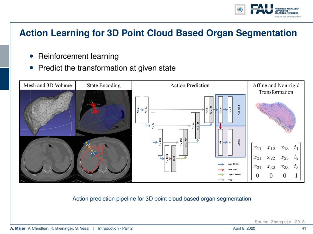
Now, this approach of prediction of organ positions from only surface information can also be used to perform organ segmentation in interventional CT. So, the idea here is that you start with an initial point-cloud of the organ and then refine it similar to the previous agent-based approach. We modify the mesh step-by-step such that it matches the organ shape in a particular image. So here you see some preoperative CT image on the left and from this, we can train algorithms and produce point clouds.
Then you can train a network that operates a deformation on those point clouds and produces new shapes such that they match the actual image appearance. Now the interesting thing about this is that this approach is pre-informed about the organ shape and does only slight changes to the organ in order to match the current image. This allows us to produce very fast and very accurate organ segmentation in interventional data. So, we train with regular CT data, but it will then also work on images that are done with a mobile C-arm or an angiography system that has a much lower image quality. These images are used in interventional settings for guidance purposes. We can apply our method in let’s say 0.3 to 2.6 seconds and this is approximately 50 to 100 times faster than a conventional U-Net approach where you do full 3-D processing.
So, next time in deep learning we will talk a bit about not just the successes, but also the limitations of deep learning. Furthermore, we also want to discuss a couple of future directions that may help to reduce these limitations. So, thank you very much for watching and hope to see you in the next video.
If you liked this post, you can find more essays here, more educational material on Machine Learning here, or have a look at our Deep Learning Lecture. I would also appreciate a clap or a follow on YouTube, Twitter, Facebook, or LinkedIn in case you want to be informed about more essays, videos, and research in the future. This article is released under the Creative Commons 4.0 Attribution License and can be reprinted and modified if referenced.
References
[1] David Silver, Julian Schrittwieser, Karen Simonyan, et al. “Mastering the game of go without human knowledge”. In: Nature 550.7676 (2017), p. 354.
[2] David Silver, Thomas Hubert, Julian Schrittwieser, et al. “Mastering Chess and Shogi by Self-Play with a General Reinforcement Learning Algorithm”. In: arXiv preprint arXiv:1712.01815 (2017).
[3] M. Aubreville, M. Krappmann, C. Bertram, et al. “A Guided Spatial Transformer Network for Histology Cell Differentiation”. In: ArXiv e-prints (July 2017). arXiv: 1707.08525 [cs.CV].
[4] David Bernecker, Christian Riess, Elli Angelopoulou, et al. “Continuous short-term irradiance forecasts using sky images”. In: Solar Energy 110 (2014), pp. 303–315.
[5] Patrick Ferdinand Christ, Mohamed Ezzeldin A Elshaer, Florian Ettlinger, et al. “Automatic liver and lesion segmentation in CT using cascaded fully convolutional neural networks and 3D conditional random fields”. In: International Conference on Medical Image Computing and Computer-Assisted Springer. 2016, pp. 415–423.
[6] Vincent Christlein, David Bernecker, Florian Hönig, et al. “Writer Identification Using GMM Supervectors and Exemplar-SVMs”. In: Pattern Recognition 63 (2017), pp. 258–267.
[7] Florin Cristian Ghesu, Bogdan Georgescu, Tommaso Mansi, et al. “An Artificial Agent for Anatomical Landmark Detection in Medical Images”. In: Medical Image Computing and Computer-Assisted Intervention – MICCAI 2016. Athens, 2016, pp. 229–237.
[8] Jia Deng, Wei Dong, Richard Socher, et al. “Imagenet: A large-scale hierarchical image database”. In: Computer Vision and Pattern Recognition, 2009. CVPR 2009. IEEE Conference IEEE. 2009, pp. 248–255.
[9] A. Karpathy and L. Fei-Fei. “Deep Visual-Semantic Alignments for Generating Image Descriptions”. In: ArXiv e-prints (Dec. 2014). arXiv: 1412.2306 [cs.CV].
[10] Alex Krizhevsky, Ilya Sutskever, and Geoffrey E Hinton. “ImageNet Classification with Deep Convolutional Neural Networks”. In: Advances in Neural Information Processing Systems 25. Curran Associates, Inc., 2012, pp. 1097–1105.
[11] Joseph Redmon, Santosh Kumar Divvala, Ross B. Girshick, et al. “You Only Look Once: Unified, Real-Time Object Detection”. In: CoRR abs/1506.02640 (2015).
[12] J. Redmon and A. Farhadi. “YOLO9000: Better, Faster, Stronger”. In: ArXiv e-prints (Dec. 2016). arXiv: 1612.08242 [cs.CV].
[13] Joseph Redmon and Ali Farhadi. “YOLOv3: An Incremental Improvement”. In: arXiv (2018).
[14] Frank Rosenblatt. The Perceptron–a perceiving and recognizing automaton. 85-460-1. Cornell Aeronautical Laboratory, 1957.
[15] Olga Russakovsky, Jia Deng, Hao Su, et al. “ImageNet Large Scale Visual Recognition Challenge”. In: International Journal of Computer Vision 115.3 (2015), pp. 211–252.
[16] David Silver, Aja Huang, Chris J. Maddison, et al. “Mastering the game of Go with deep neural networks and tree search”. In: Nature 529.7587 (Jan. 2016), pp. 484–489.
[17] S. E. Wei, V. Ramakrishna, T. Kanade, et al. “Convolutional Pose Machines”. In: CVPR. 2016, pp. 4724–4732.
[18] Tobias Würfl, Florin C Ghesu, Vincent Christlein, et al. “Deep learning computed tomography”. In: International Conference on Medical Image Computing and Computer-Assisted Springer International Publishing. 2016, pp. 432–440.