From Spectral to Spatial Domain
These are the lecture notes for FAU’s YouTube Lecture “Deep Learning“. This is a full transcript of the lecture video & matching slides. We hope, you enjoy this as much as the videos. Of course, this transcript was created with deep learning techniques largely automatically and only minor manual modifications were performed. Try it yourself! If you spot mistakes, please let us know!
Welcome back to deep learning. So today, we want to continue talking about graph convolutions. We will look into the second part where we now see whether we have to stay in this spectral domain or whether we can also go back to the spatial domain. So let’s look at what I have for you.
Remember we had this polynomial to define a convolution in the spectral domain. We’ve seen that by computing the eigenvectors of the Laplacian matrix, we were able to find an appropriate Fourier transform that would then give us a spectral representation of the graph configuration. Then, we could do our convolution in the spectral domain and transform it back. Now, this was kind of very expensive because we have to compute U. For U, we have to do the eigenvalue decomposition for this entire symmetric matrix. Also, we’ve seen that we can’t use tricks of the fast Fourier transform because this doesn’t necessarily hold for our U.
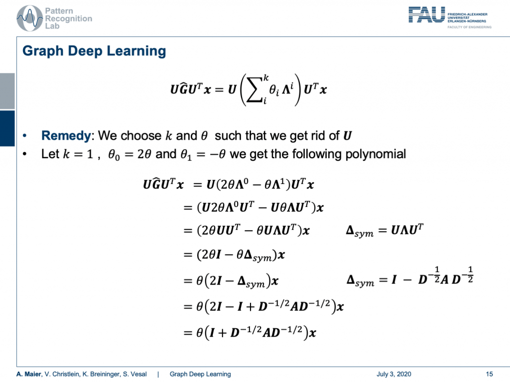
So, how can we choose now our k and θ in order to get rid of U? Well, so if we choose k equals to 1, θ subscript 0 to 2θ, and θ subscript 1 to -θ, we get the following polynomial. So, we still have the configuration that we have x transformed in the Fourier space times our polynomial expressed as matrix times the inverse Fourier transform here. Now, let’s look into the configuration of G hat. G hat can actually be expressed as 2 times θ times Λ to the power of 0. Remember Λ is a diagonal matrix. So, we take every element to the power of 0. This is actually a unity matrix and we subtract θ times Λ to the power of 1. Well, this is actually just Λ. Then, we can express our complete matrix G hat in this way. Of course, we can then pull in our U from the left-hand side and the right-hand side which is giving us the following expression. Now, we use the property that θ is actually a scalar. So, we can pull it to the front. The Λ to the power of 0 cancels out because this is essentially an identity matrix. The Λ on the right-hand side term still remains, but we can also pull out the θ. Well the UU transpose just cancels out. So, this is again the identity matrix and we can use our definition of the symmetric version of our graph Laplacian. You can see that we’ve just found it, here in our equation. So, we can also replace it with this one. You see now U is suddenly gone. So, we can pull out θ again and all that remains is that we have two times the identity matrix minus the symmetric version of the graph Laplacian. If we now plug in the definition of the symmetric version associated with the original adjacency matrix and the degree matrix, we can see that we still can plug this definition in. Then, one of the identity matrices cancels out and we finally get identity plus D to the power of -0.5 times A times D to the power of -0.5. So, remember D is a diagonal matrix. We can easily invert the elements on the diagonal and we can also take element-wise the square root. So, this is perfectly fine. This way we don’t have U at all coming up here. We can express our entire graph convolution in this very nice way using the graph Laplacian matrix.
Now let’s analyze this term a little more. So, we can see this identity on the left-hand side, we see we can convolve in the spectral domain, and we can construct G hat as a polynomial of Laplacian filters. Then, we can see with a particular choice k equals 1, θ subscript 0 equals to 2θ and θ subscript 1 equals to -θ. Then, this term suddenly only depends on the scalar value θ. With all these tricks, we got rid of the Fourier transform U transpose. So, we suddenly can express graph convolutions in this simplified way.
Well, this is the basic graph convolutional operation and you can find this actually shown in reference [1]. You can essentially do this to scalar values, you use your degree matrix and plug it in here. You use your adjacency matrix and you plug it in here. Then, you can optimize with respect to θ in order to find the weight for your convolutions.
Well, now the question is “Is it really necessary to motivate the graph convolution from the spectral domain?” and the answer is “No.”. So, we can also motivate it spatially.
Well, let’s look at the following concept. For a mathematician, a graph is a manifold, but a discrete one. We can discretize the manifold and do a spectral convolution using the Laplacian matrix. So, this led us to spectral graph convolutions. But as a computer scientist, you can interpret a graph as a set of nodes and vertices connected through edges. We now need to define how to aggregate the information of one vertex through its neighbors. If we do so, we get the spatial graph convolution.
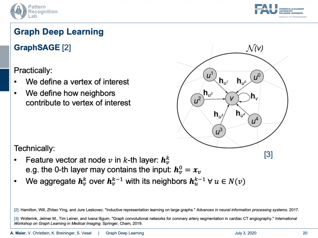
Well, how is this done? One approach shown in [2] is GraphSAGE. Here, we essentially define a vertex of interest and we define how neighbors contribute to the vertex of interest. So technically, we implement this using a feature vector at the node v and the k-th layer. This can be described as h k subscript v. So, for the zeroth layer, this contains the input. This is just the original configuration of your graph. Then, we need to be able to aggregate in order to compute the next layer. This is done by a spatial aggregation function over the previous layer. Therefore, you use all of the neighbors and typically you define this neighborhood such that every node that is connected to the node under consideration is included in this neighborhood.
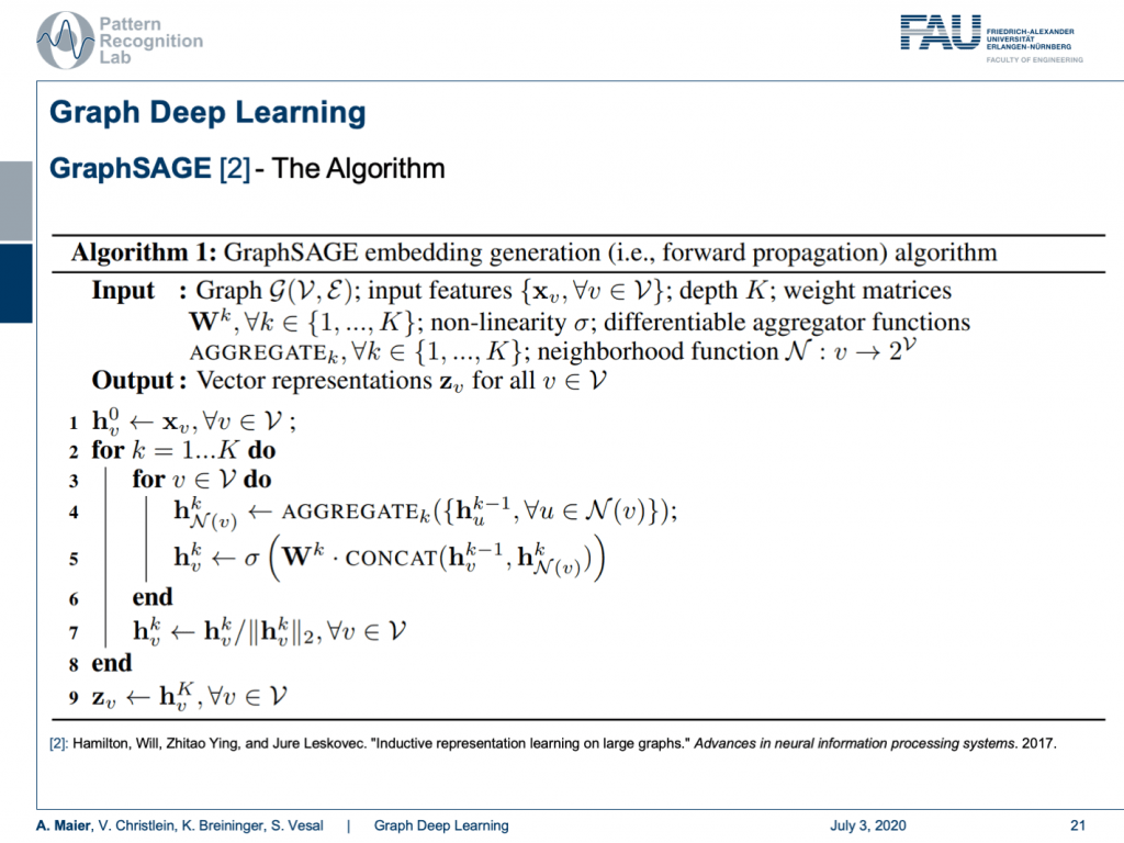
So this line brings us to the GraphSAGE algorithm. Here, you start with a graph and input features. Then, you do the following algorithm: You initialize at h 0 with simply the input of the graph configuration. Then, you iterate over the layers. You iterate over the nodes. For every node, you run the aggregation function that somehow computes a summary over all of your neighbors. Then, the result is a vector of a certain dimension and you then take the aggregated vector and the current configuration of the vector, you concatenate them and multiply them with a weight matrix. This is then run through a non-linearity. Lastly, you scale by the magnitude of your activations. This is then iterated over all of the layers and finally, you get the output z that is the result of your graph convolution.
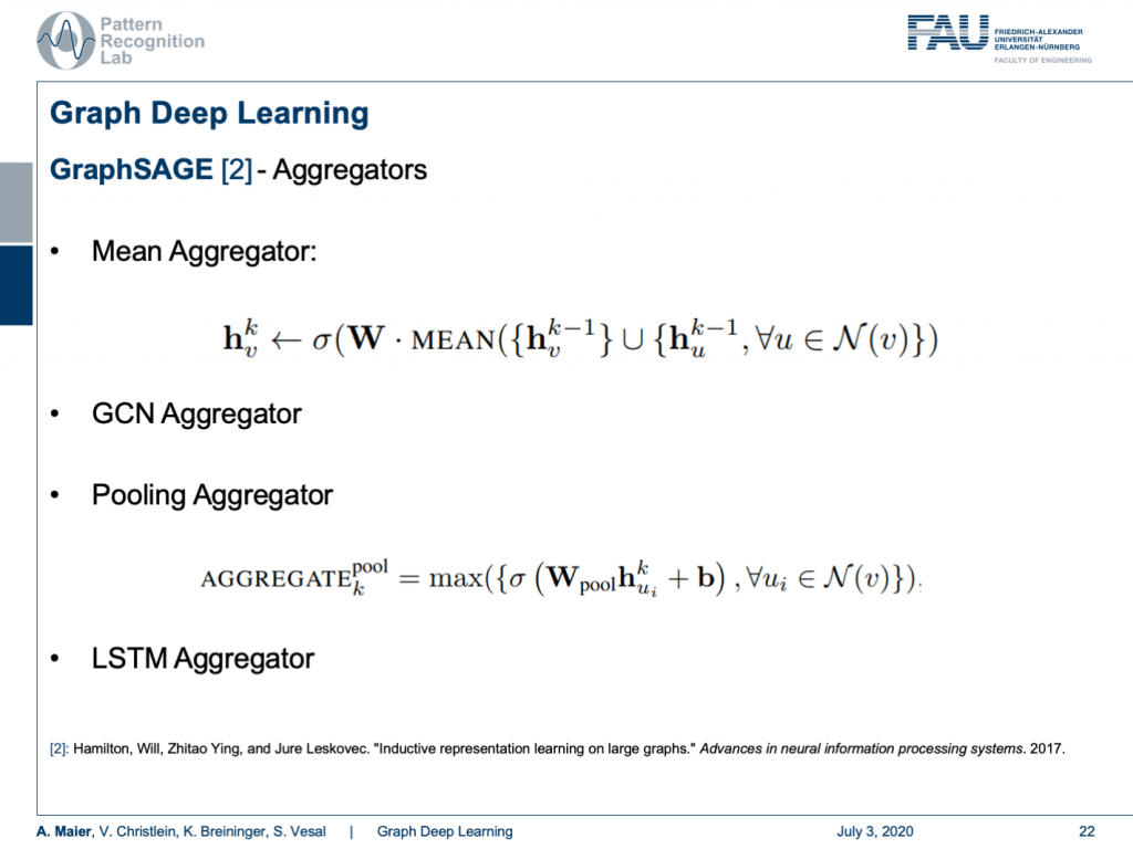
The concept of aggregators is key to develop this algorithm because in every node you may have a different number of neighbors. A very simple aggregator would then be simply computing the mean. Of course, you can also take the GCN aggregator and that brings us back to the spectral representation. This way, the connection between spatial and spectral domains can be established. Furthermore, you can take a pooling aggregator which then uses, for example, maximum pooling or you use recurrent networks like LSTM aggregators.
You already see that there is a broad variety of aggregators. This then also is the reason why there are so many different graph deep learning approaches. You can subdivide them into certain kinds because there are spectral ones, there are spatial ones, and there are the recurrent ones. So, this is essentially the key how you can tackle the graph convolutional neural networks. So, what do we actually want to do? Well, you can take one of these algorithms and apply it to some mesh. Of course, this can also be done on very complex meshes and I will put a couple of references below that you can see what kind of applications can be done. For example, you can use these methods in order to process the information on coronary arteries.
Well next time in deep learning, there’s only a couple of topics left. One thing that I want to show to you is how you can embed prior knowledge into deep networks. This is also a quite nice idea because it allows us to fuse much of the things that we know from theory and signal processing with our deep learning approaches. Of course, I also have a couple of references and if you have some time please read through them. They elaborate much more closely on the ideas that we presented here. There are also image references that I’ll put into the description of this video. So, thank you very much for listening and see you in the next lecture. Bye-bye!
If you liked this post, you can find more essays here, more educational material on Machine Learning here, or have a look at our Deep LearningLecture. I would also appreciate a follow on YouTube, Twitter, Facebook, or LinkedIn in case you want to be informed about more essays, videos, and research in the future. This article is released under the Creative Commons 4.0 Attribution License and can be reprinted and modified if referenced. If you are interested in generating transcripts from video lectures try AutoBlog.
Thanks
Many thanks to the great introduction by Michael Bronstein on MISS 2018! and special thanks to Florian Thamm for preparing this set of slides.
References
[1] Kipf, Thomas N., and Max Welling. “Semi-supervised classification with graph convolutional networks.” arXiv preprint arXiv:1609.02907 (2016).
[2] Hamilton, Will, Zhitao Ying, and Jure Leskovec. “Inductive representation learning on large graphs.” Advances in neural information processing systems. 2017.
[3] Wolterink, Jelmer M., Tim Leiner, and Ivana Išgum. “Graph convolutional networks for coronary artery segmentation in cardiac CT angiography.” International Workshop on Graph Learning in Medical Imaging. Springer, Cham, 2019.
[4] Wu, Zonghan, et al. “A comprehensive survey on graph neural networks.” arXiv preprint arXiv:1901.00596 (2019).
[5] Bronstein, Michael et al. Lecture “Geometric deep learning on graphs and manifolds” held at SIAM Tutorial Portland (2018)
Image References
[a] https://de.serlo.org/mathe/funktionen/funktionsbegriff/funktionen-graphen/graph-funktion
[b] https://www.nwrfc.noaa.gov/snow/plot_SWE.php?id=AFSW1
[c] https://tennisbeiolympia.wordpress.com/meilensteine/steffi-graf/
[d] https://www.pinterest.de/pin/624381935818627852/
[e] https://www.uihere.com/free-cliparts/the-pentagon-pentagram-symbol-regular-polygon-golden-five-pointed-star-2282605
[f] http://geometricdeeplearning.com/ (Geometric Deep Learning on Graphs and Manifolds)
[g] https://i.stack.imgur.com/NU7y2.png
[h] https://de.wikipedia.org/wiki/Datei:Convolution_Animation_(Gaussian).gif
[i]https://www.researchgate.net/publication/306293638/figure/fig1/AS:396934507450372@1471647969381/Example-of-centerline- extracted-left-and-coronary-artery-tree-mesh-reconstruction.png
[j] https://www.eurorad.org/sites/default/files/styles/figure_image_teaser_large/public/figure_image/2018-08/0000015888/000006.jpg?itok=hwX1sbCO