Lecture Notes in Deep Learning: Graph Deep Learning – Part 1

Spectral Convolutions

These are the lecture notes for FAU’s YouTube Lecture “Deep Learning“. This is a full transcript of the lecture video & matching slides. We hope, you enjoy this as much as the videos. Of course, this transcript was created with deep learning techniques largely automatically and only minor manual modifications were performed. Try it yourself! If you spot mistakes, please let us know!

Welcome back to deep learning! So today, we want to look a bit into how to process graphs and we will talk a bit about graph convolutions. So let’s see what I have here for you. Topic today will be an introduction to graph deep learning.

Well, what’s graph deep learning? You could say this is a graph, right? We know that from math that we can plot graphs. But this is not what we’re going to talk about today. Also, you could say a graph is like a plot like this one. But these are also not the plots that we want to talk about today. So is it Steffi Graf? No, we are also not talking about Steffi Graf. So what we actually want to look at are more things like this like diagrams that can be connected with different nodes and edges.

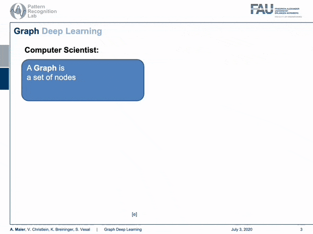
A computer scientist thinks of a graph as a set of nodes and they are connected through edges. So this is the kind of graph that we want to talk about today. For a mathematician, a graph is a manifold, but a discrete one.

Now, how would you define a convolution? On euclidean space, well both for computer scientists and mathematicians this is too easy. So this is the discrete convolution which is essentially just a sum. We remember we had many of those discrete convolutions when we are setting up the kernels for our convolutional deep models. In the continuous form, it actually takes the following form: It’s essentially an integral that is computed over the entire space and I brought an example here. So if you want to convolve two Gaussian curves, then you essentially move them over each other multiply at each point and sum them up. Of course, the convolution of two Gaussians is a Gaussian again so this is also easy.

How would you define a convolution on graphs? Now, the computer scientist thinks really hard but … What the heck! Well, the mathematician knows that we can use Laplace transforms in order to describe convolutions and therefore we look into the laplacian that is here given as the divergence of the gradient. So in math, we can deal with these things more easily.

This then brings us to this manifold idea. We know how to convolve manifolds, we can discretize convolutions, and this means that we know how to convolve graphs.

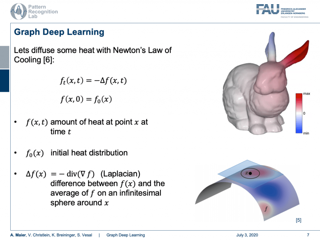
So, let’s diffuse some heat! We know that we can describe Newton’s law of cooling as the following equation. We also know that the development over time can be described with the Laplacian. So, f(x,t) is then the amount of heat at point x at time t. Then, you need to have an initial heat distribution. So, you need to know how the heat is in the initial state. Then, you can use the Laplacian in order to express how the system behaves over time. Here, you can see that this is essentially the difference between f(x) and the average of f on an infinite decimal small sphere around x.

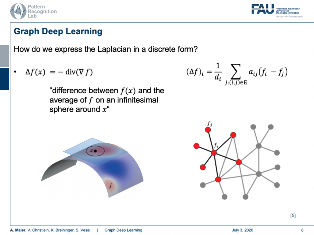
Now, how do we express the Laplacian in discrete form? Well, that’s the difference between f(x) and the average of f on an infinitesimal sphere around x. So, the smallest step that we can do is actually connect the current node with its neighbors. So, we can express the Laplacian as a weighted sum over the edge weights a subscript i and j. This is then the difference of our center node f subscript i minus f subscript j and we divide the whole thing by the number of connections that actually are incoming into f subscript i. This is going to be given as d subscript i.

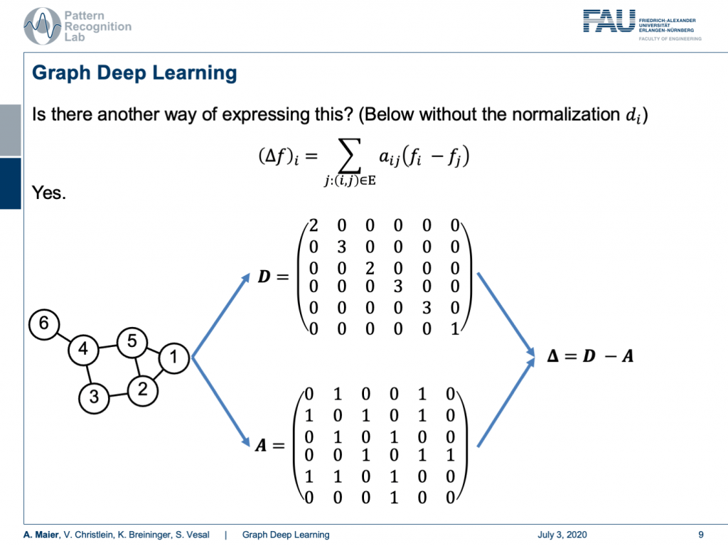
Now is there another way of expressing this? Well, yes. We can do this if we look at an example graph here. So, we have the nodes 1, 2, 3, 4, 5, and 6. We can now compute the Laplacian matrix using the matrix D. D is now simply the number of incoming connections into the respective nodes. So, we can see that Node 1 has two incoming connections, Node 2 has three, Node 3 has two, Node 4 has three, and Node 5 also has three, Node 6 has only one incoming connection. What we else need is the matrix A. That’s the adjacency matrix. So here, we have a 1 for every node that is connected with a different node and you can see it can be expressed with the above matrix now. We can take the two and compute the Laplacian as D minus A. We simply element-wise subtract the two to get our Laplacian matrix. This is nice.

We can see that the Laplacian is an N times N matrix and it’s describing a graph or subgraph consisting of N nodes. D is also an N times N matrix and it’s called the degree matrix and describes the number of edges connected to each node. A is also an N times N matrix and it’s the adjacency matrix that describes the connectivity of the graph. So for a directed graph, our graph Laplacian matrix is not symmetric positive definite. So, we need to normalize it in order to get a symmetric version. This can be done in the following way: We start with the original Laplacian matrix. We know that D is simply a diagonal matrix. So, we can compute the inverse square root and multiply it from the left-hand side and right-hand side. Then, we can plug in the original definition and you see that we can rearrange this a little bit. We can then write the symmetrized version as the unity matrix minus D. Here, we apply again element-wise the inverse and the square root times A times the same matrix. So this is very interesting, right? We can always get the symmetrized version of this matrix even for directed graphs.

Now, we are interested in how to use this actually. We can do some magic and the magic now is if our matrix is symmetric positive definite, then the matrix can be decomposed into eigenvectors and eigenvalues. Here, we see that all the eigenvectors are assembled in U and the eigenvalues are on this diagonal matrix Λ. Now, these eigenvectors are known as the graph Fourier modes. The eigenvalues are known as spectral frequencies. This means that we can use U and U transpose in order to Fourier transform a graph and our Λ are the spectral filter coefficients. So, we can transform a graph into a spectral representation and look at its spectral properties.

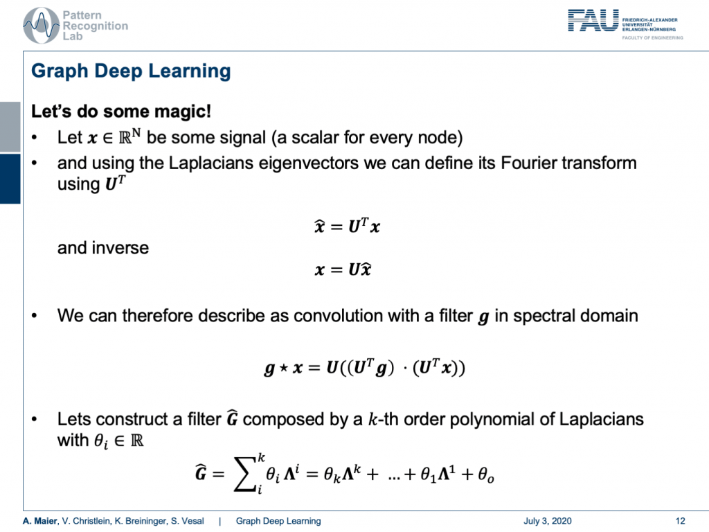
Let’s continue with our matrix. Now, let x be some signal, a scalar for every node. Then, we can use the Laplacian’s eigenvectors to define its Fourier transform. This then is simply x hat and x hat can be expressed as U transposed times x. Of course, you can also invert this. This is simply done by applying U. So, we can also find for any set of coefficients that are describing properties of the nodes, the respective spectral representation. Now, we can also describe a convolution with a filter in the spectral domain. So, we express the convolution using a Fourier representation and therefore we bring g and x into Fourier domain, multiply the two and compute the inverse Fourier transform. So, we know that from signal processing that we can also do this in traditional signals.

Now, let’s construct a filter. This filter is composed of a k-th order polynomial of Laplacians with coefficients θ subscript i. They are simply real numbers. So, we can now find this kind of polynomial that is a polynomial with respect to the spectral coefficients and it’s linear in the coefficients θ. This is essentially just a sum over the polynomials. So now, we can use that and use this filter in order to perform our convolution. We essentially have to multiply in the same way as we did before. So, we have the signal, we apply the Fourier transform, then we apply our convolution using our polynomial, and then we do the inverse Fourier transform. So, this would be how we would apply this filter to a new signal. And now, what? Well, we can convolve x now using the laplacian as we adapt our filter coefficients θ. But U is actually really heavy. Remember we can’t use the trick of a fast Fourier transform here. So, it’s always a full matrix multiplication and this might be very heavy to compute if you want to express your convolutions in this type of format. But what if I told you that a clever choice of polynomials cancels out U entirely?

Well, this is what we will discuss in the next session on deep learning. So, thank you very much for listening so far and see you in the next video. Bye-bye!

If you liked this post, you can find more essays here, more educational material on Machine Learning here, or have a look at our Deep LearningLecture. I would also appreciate a follow on YouTube, Twitter, Facebook, or LinkedIn in case you want to be informed about more essays, videos, and research in the future. This article is released under the Creative Commons 4.0 Attribution License and can be reprinted and modified if referenced. If you are interested in generating transcripts from video lectures try AutoBlog.

Thanks

Many thanks to the great introduction by Michael Bronstein on MISS 2018 and special thanks to Florian Thamm for preparing this set of slides.

References

[1] Kipf, Thomas N., and Max Welling. “Semi-supervised classification with graph convolutional networks.” arXiv preprint arXiv:1609.02907 (2016).
[2] Hamilton, Will, Zhitao Ying, and Jure Leskovec. “Inductive representation learning on large graphs.” Advances in neural information processing systems. 2017.
[3] Wolterink, Jelmer M., Tim Leiner, and Ivana Išgum. “Graph convolutional networks for coronary artery segmentation in cardiac CT angiography.” International Workshop on Graph Learning in Medical Imaging. Springer, Cham, 2019.
[4] Wu, Zonghan, et al. “A comprehensive survey on graph neural networks.” arXiv preprint arXiv:1901.00596 (2019).
[5] Bronstein, Michael et al. Lecture “Geometric deep learning on graphs and manifolds” held at SIAM Tutorial Portland (2018)

Image References

[a] https://de.serlo.org/mathe/funktionen/funktionsbegriff/funktionen-graphen/graph-funktion
[b] https://www.nwrfc.noaa.gov/snow/plot_SWE.php?id=AFSW1
[c] https://tennisbeiolympia.wordpress.com/meilensteine/steffi-graf/
[d] https://www.pinterest.de/pin/624381935818627852/
[e] https://www.uihere.com/free-cliparts/the-pentagon-pentagram-symbol-regular-polygon-golden-five-pointed-star-2282605
[f] http://geometricdeeplearning.com/ (Geometric Deep Learning on Graphs and Manifolds)
[g] https://i.stack.imgur.com/NU7y2.png
[h] https://de.wikipedia.org/wiki/Datei:Convolution_Animation_(Gaussian).gif
[i]https://www.researchgate.net/publication/306293638/figure/fig1/AS:396934507450372@1471647969381/Example-of-centerline- extracted-left-and-coronary-artery-tree-mesh-reconstruction.png
[j] https://www.eurorad.org/sites/default/files/styles/figure_image_teaser_large/public/figure_image/2018-08/0000015888/000006.jpg?itok=hwX1sbCO

Category: Lecture Notes in Deep Learning