Lecture Notes in Deep Learning: Feedforward Networks – Part 3

The Backpropagation Algorithm

These are the lecture notes for FAU’s YouTube Lecture “Deep Learning“. This is a full transcript of the lecture video & matching slides. We hope, you enjoy this as much as the videos. Of course, this transcript was created with deep learning techniques largely automatically and only minor manual modifications were performed. If you spot mistakes, please let us know!

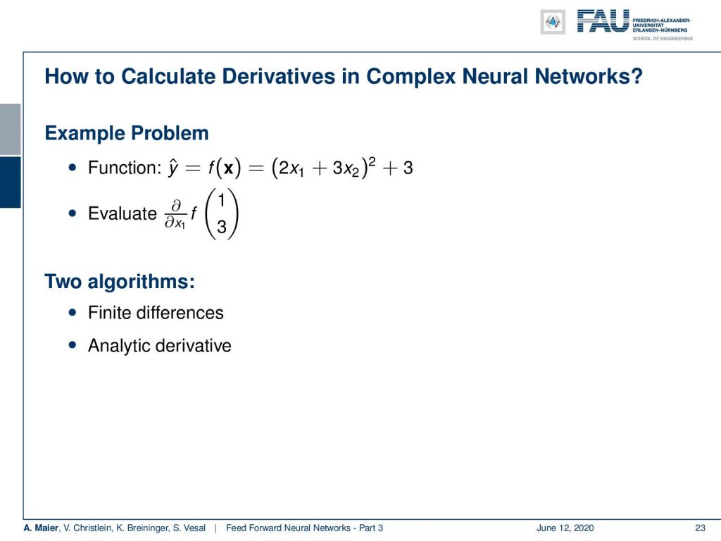
Welcome everybody to deep learning! Thanks for tuning in. Today’s topic will be the backpropagation algorithm. So, you may be interested in how we actually compute these derivatives in complex neural networks. Let’s look at a simple example. Our true function is 2 x₁ plus 3 x₂ to the power of 2 plus 3. Now, we want to evaluate the partial derivative of f(x) at the position (1 3)ᵀ with respect to x₁. There are two algorithms that can do that quite efficiently. The first one will be finite differences. The second one is an analytic derivative. So, we will go through both examples here.

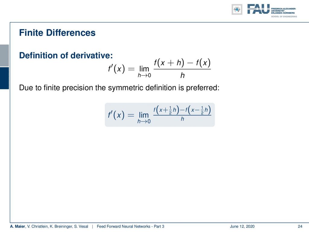
For finite differences, the idea is that you compute the function value at some position x. Then, you add a very small increment h to x and evaluation the function there. You also compute the at function f(x) and take the difference between the two. Then, you divide by the value of h. So this is actually the definition of a derivative: It is the limit of the difference between f(x+h) and f(x) divided by h in which we let h approach 0. Now, the problem is this is not symmetric. So, sometimes you want to prefer a symmetric definition. Instead of computing this exactly at x, we go h/2 back and h/2 to the front. This allows us to compute the derivative exactly at the position x. Then, we still have to divide over h. This is a symmetric definition.

We can do this for our example. Let’s try to evaluate this. We take our original definition (2x₁+ 3x₂)² + 3. We wanted to look at the position (1 3)ᵀ. Let’s use the +h/2 definition above. Here, we set h to a small value, say 2 ⋅ 10⁻². We plug it in and you can see that here in this row. So this is going to be ((2(1+10⁻²+9)² + 3) and of course, we also have to subtract our small value in the second term. Then, we divide by the small value as well. So, we will end up with approximately 124.4404 minus 123.5604. This will be approximately 43.9999. So, we can compute this for any function, even if we don’t know the definition of the function, e.g., if one only has as a software module that we cannot access. In this case, we can use finite differences to approximate the partial derivative.

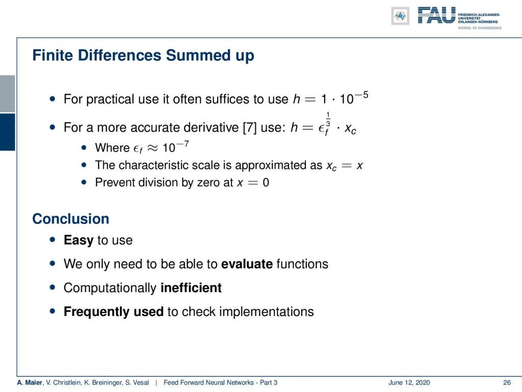
Practically, use we use h in the range of 1⋅ 10⁻⁵ which is appropriate for floating-point precision. Depending on the precision of your computing system, you can also determine what the appropriate value for h is going to be. You can check that in reference number seven. We see that this is really easy to use. We can evaluate this on any function we don’t need to know the formal definition, but of course, it’s computationally inefficient. Imagine you want to determine the gradient that is the set of all partial derivatives of a function that has a dimension of 100. This means that you have to evaluate the function 101 times to compute this entire gradient. So, this may not be such a great choice for general optimization, because it may become inefficient. But of course, it’s a very cool method to check your implementation. Imagine you implemented the analytic version and sometimes you make mistakes. Then, you can use this as a trick to check whether your analytic derivative is correctly implemented. This is also something you will learn in detail in the exercises here. It’s really useful if you want to debug your implementation.

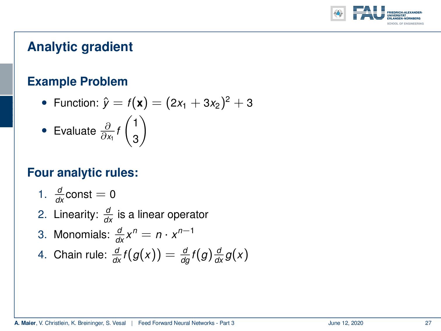
Okay, so let’s talk about analytic gradients. Now the analytic gradient, we can derive by using a set of analytic differentiation rules. So, the first rule is going to be the derivative of a constant is going to be 0. Then, our operator is a linear operator which means we can rearrange it if we have for example sums of different components. Next, we also know the derivatives of monomials. If you have some xⁿ, the derivative is going to be n ⋅ xⁿ⁻¹. The chain rule applies if you have nested functions. It’s essentially the key idea that we also need for the backpropagation algorithm. You see that the derivative with respect to x of some nested function is going to be the derivative of the function with respect to g multiplied with the derivative of the function g with respect to x.

Ok so let’s place those to the very top right. We will need them in the next couple of slides. Let’s try to calculate this so here you see that partial derivative with respect to x₁ of f(x) at (1 3)ᵀ. Then, we can just plug in the definition. So, this is going to be the partial derivative of (2x₁+9)². So, we can already write the 9, because so we can already plug in the 3 and multiply it with 3 to obtain 9. In the next step, we can essentially compute the partial derivative with respect to the outer function. Now. there’s the application of the chain rule and we introduce this new variable z. In the next step, we can then compute the partial derivative of z to the power of 2, where we have to reduce the exponent by 1 and then multiply with this exponent. So, this is going to be 2(2x₁+9) times the partial derivative of 2x₁+9. So, we can simplify this a little bit further. You can see that if we apply the partial derivative on the 2x₁+9, x₁ cancels away. Only 2 remains as minus the constant 9 also vanishes. So in the end, we end up with 2(2x₁+9) times 2. Now if you plug in x₁ = 1, you will see that our derivative equals to 44. In our numerical implementation that we have evaluated previously, you can see that we had 43.9999. So, we were pretty close. But of course, the analytic gradient is more accurate.

Now the question is: “Can we do this automatically?” and of course the answer is “yes”. We use those rules, the chain rule, linearity, and the other two to decompose the complex functions of neural networks. We don’t do that manually but we do it completely automatically in the backpropagation algorithm. This is going to be more computationally efficient than finite differences.

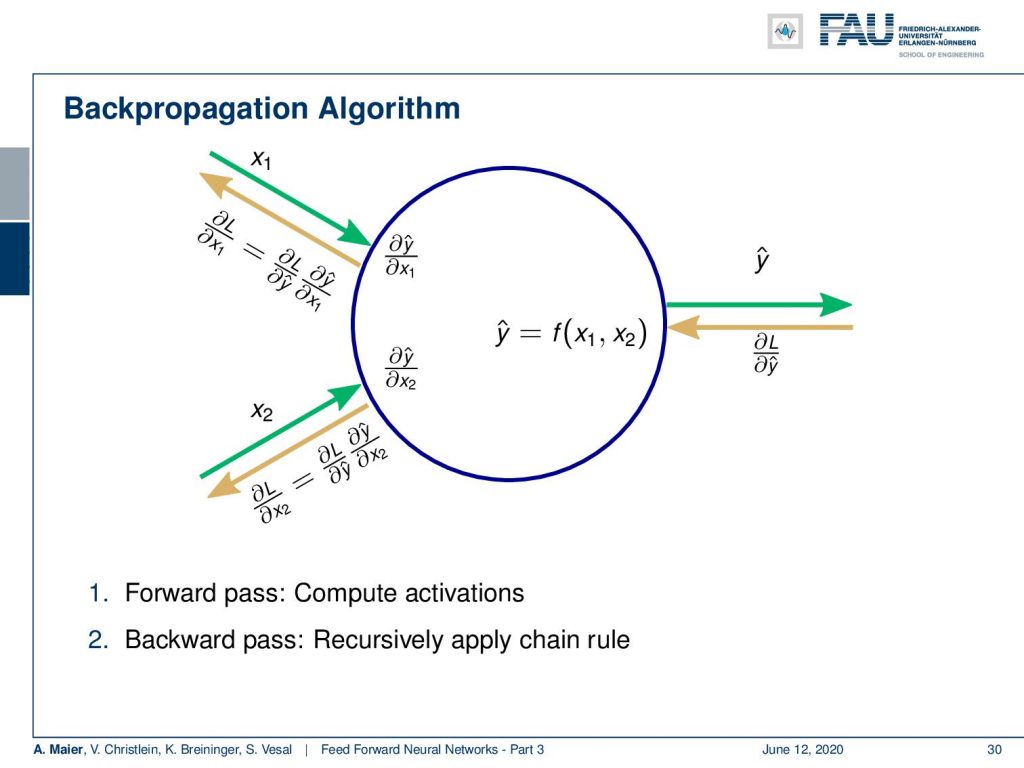
So, you can essentially describe the backpropagation algorithm in a nutshell here: For every neuron, you need to have the inputs x₁, x₂, and of course the output that is y hat. Then, you can compute – in green – the forward pass. You evaluate somewhere the loss function and you get the derivative with respect to y hat that comes in in the backward pass. Then, for every element in your network graph, you need to know the derivatives with respect to the inputs, here x₁ and x₂. What we’re missing in this figure are, of course, trainable weights. For trainable weights, we would then also need to compute the derivatives with respect to them, in order to compute the parameter updates. So, for every module or node, you need to know the derivative with respect to the inputs and the derivative with respect to the weights. If you have that for every module then you can compose a graph and with this graph, you can then compute arbitrary derivatives of very complex functions.

Let’s go back to our example and apply backpropagation to it. So, what do we do? Well, we compute the forward pass first. In order to be able to compute the forward pass, we plug in intermediate definitions. So we decompose this now into some a that is 2 times x₁ and b that is 3 times x₂. Then, we can compute those: We get the values 2 and 9 for a and b. This allows us to compute c that is the sum of the two. This equates to 11. Then, we can compute e from that that is nothing else than the power of 2 of c. This gives us 121 and now we finally compute g, that is e plus 3. So, we end up with 124.

Ok, now we need to backpropagate. So, we need to compute the partial derivatives. Here, the partial derivatives of g with respect to e is going to be 1. Then, we compute the partial derivative of e respect to c and you’re going to see that this is 2c. With c being 11 this evaluates to 22. Then, we need a partial derivative of c with respect to a which is again 1. Now, we need the partial derivative of a with respect to x₁. If you look at this block, you can see that this partial derivative is going to be 2. So we have to multiply all the partial derivatives from right to left in order to get the result: 1 times 22 times 1 times 2 and this is going to be 44. So, this was the backpropagation algorithm applied to our example.

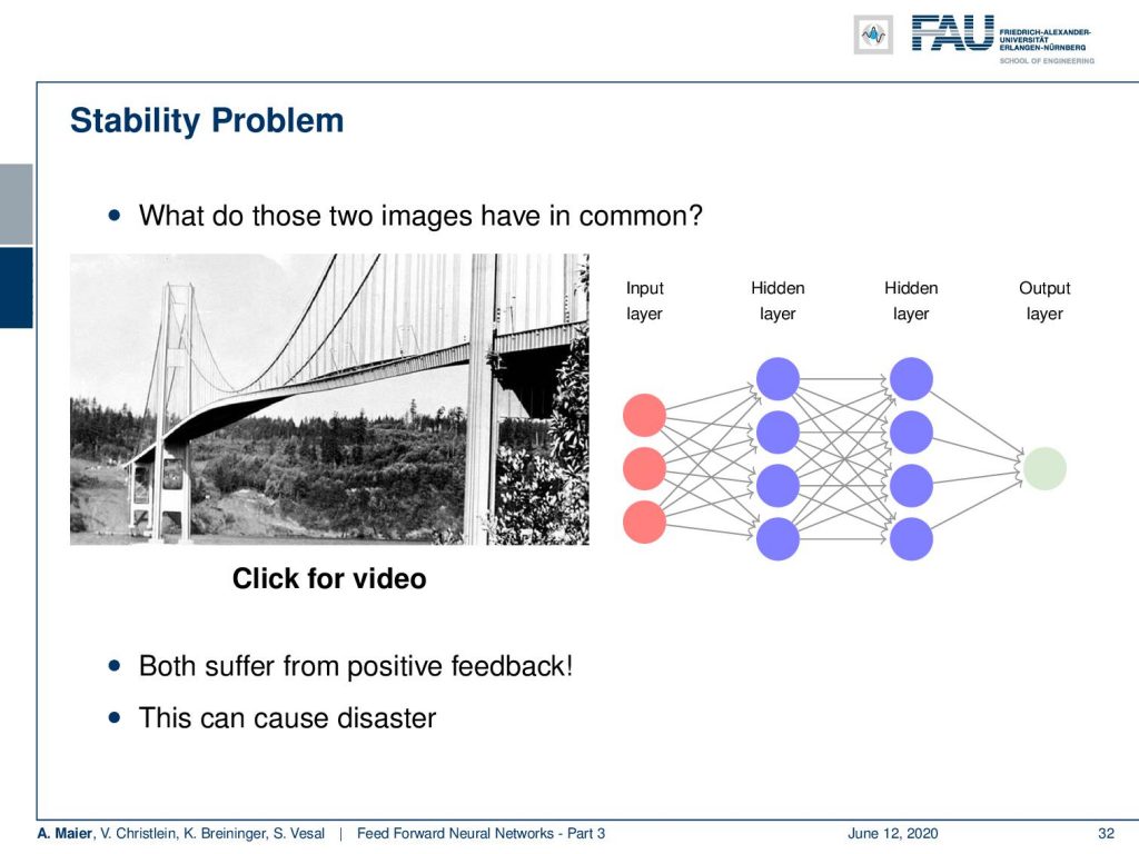
Now, we do have a kind of stability problem. We multiply with potentially high and low numbers quite frequently in the scope of the backpropagation algorithm. This then gives us the problem of positive feedback and this can cause disaster. An example of positive feedback and how it can lead to disaster is shown in the small video here.

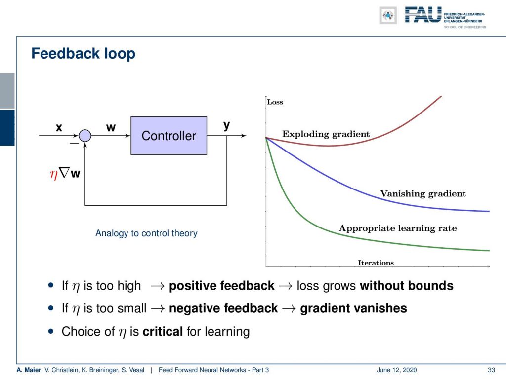
Now, what can we do about it? This is essentially a feedback loop. We have this controller and the output, where we compute the gradient. You see that there is this value of η. So, if we have η too high, it will create positive feedback. This will then result in very high values of our updates and then our loss may grow or really explode. So if it is too large, we even may have an increase in the loss function although we seek to minimize it. What can also happen is if you pick η too small, then you end up with the blue curve. That is called the vanishing gradient where we just have too small steps and we don’t get into a good convergence. So there’s no reduction of loss. It’s also a problem called “vanishing gradients”. So, only if you choose η appropriately, you will get a good learning rate. With a good learning rate, the loss should start decreasing very quickly over many iterations following this green curve. We should go then into some kind of convergence and when we have no changes anymore, we’re essentially at the point of convergence on the training data set. We can then stop updating our weights. So, we see that the choice of EDA is critical for our learning, and only if you said it appropriately you will get a good training process.

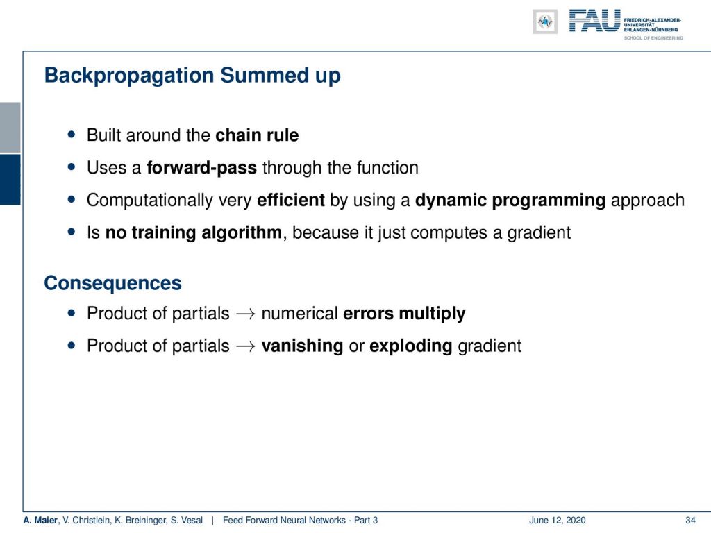
So let’s sum up backpropagation: It’s built around the chain rule. It uses a forward pass. Once we’re at the end and evaluate the loss function – essentially the difference to our learning target – then we can backpropagate. These computations are very efficient using a dynamic programming approach. Backpropagation is not a training algorithm. It is just a way of computing a gradient. You will see the actual training programs when we discuss loss and optimization in one of the next lectures. Some very important consequences are: We have a product of partials which means the numerical error is multiplied. This can be very problematic. Also because of the product of partials, we then result either in vanishing or exploding gratings. So, when you have very low values close to zero values and you start multiplying them with each other, then you have an exponential decay, causing vanishing gradients. If you have very high numbers, of course, you can also very quickly end up in an exponential growth – the exploding gradients.

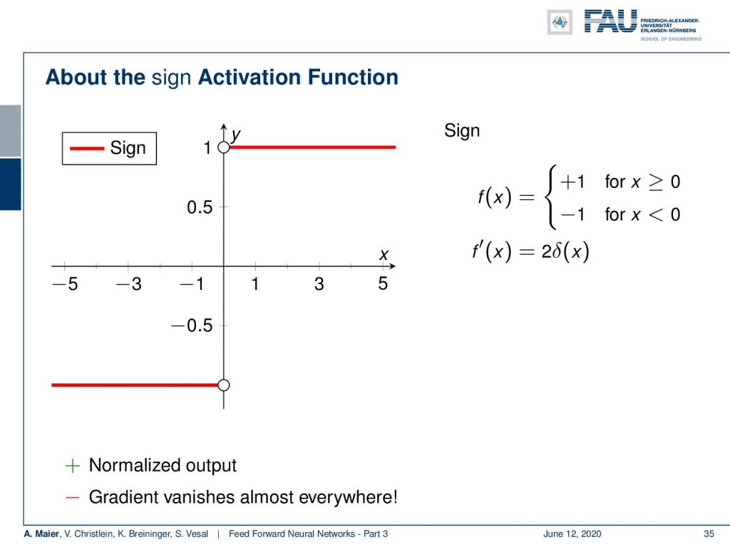
We see gradients are critical for our training. So let’s talk a bit about activation functions and their derivatives. One of the classical ones is the sign function. We already had that in the perceptron. Now, you can see that it’s symmetric and normalized between 1 and -1. But remember, we are talking about partial derivatives in order to compute the weight updates. So, the derivative of this function is a bit problematic because it’s 0 everywhere except at the point 0 and there you essentially have infinity as value. So it’s not really great to use this in combination with gradient descent.

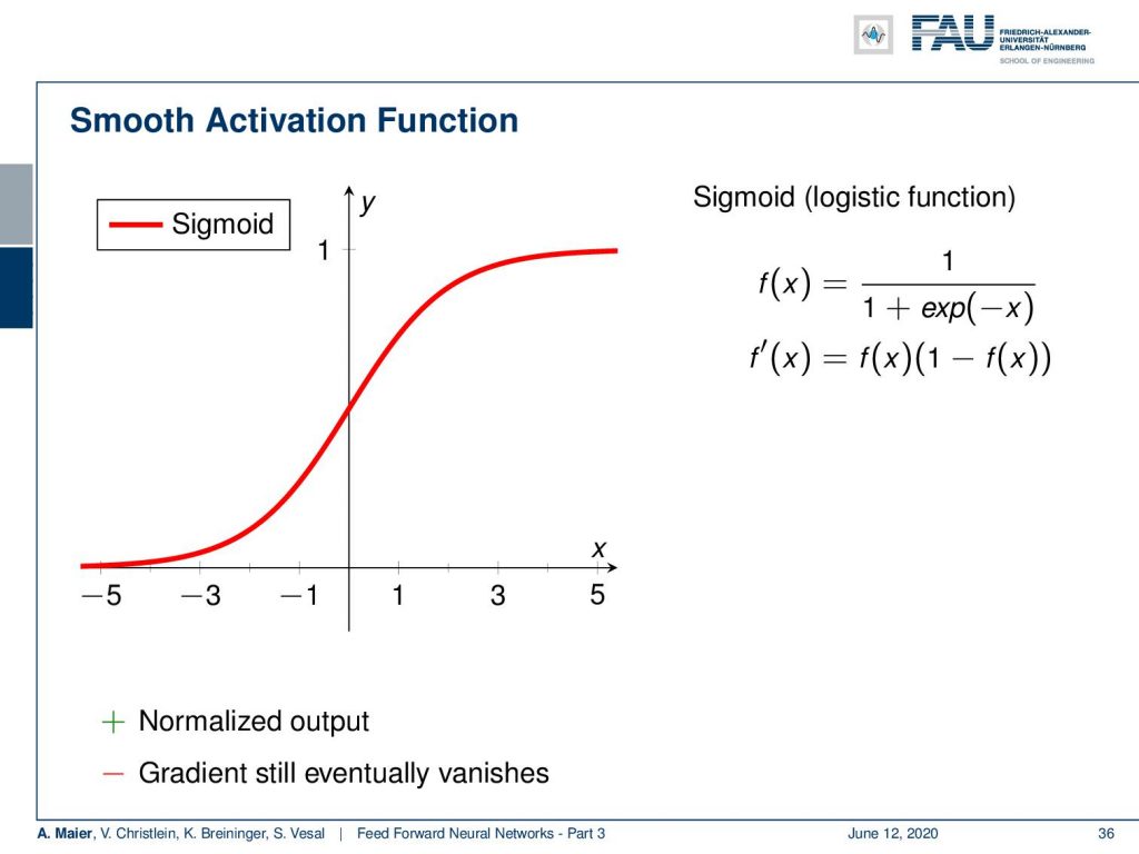
So what people have been doing? They switched to different functions and a popular one is the sigmoid function. So, it’s an s-shaped function that scales everything between 0 and 1 using a negative exponential function in the denominator. The nice thing is that if you compute the derivative of this, this is essentially f(x) times 1 – f(x). So, at least the derivative can be computed quite efficiently. In the forward pass, you always have to deal with the exponential functions which are also kind of problematic. Also, if you look at this function between let’s say between -3 and 3, you get gradients that may be suited for backpropagation. As soon as you go farther away from -3 or 3, you see that the derivative of this function will be very close to zero. So, we have saturation and again if you expect that you have a couple of those sigmoid functions behind each other, then it’s quite likely that it will produce very low values. This can also then lead to vanishing gradients.

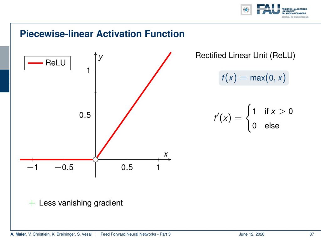
So what did people do to beat that? Well, they introduced a piecewise linear activation function called “rectified linear unit” (ReLU) which is the maximum of zero and x. So, everything that is below zero is clipped to zero and everything else is just kept. Now, this is nice because we can compute this very efficiently. There’s no exponential function involved and the derivative is simply 1 if x was greater than zero and zero everywhere else. So, there’s much less vanishing gradient as essentially the entire positive half-space can be used for gradient descent. There are also some problems with the ReLU which we will look in more detail when we talk about activation functions.

Okay, now you understood many basic concepts of the backpropagation algorithm. But we still have to talk about more complex situations and in particular layers. So right now, we did everything on the neural node level. If you want to do all of the backpropagation on neuron-level, it’s very hard and you will very quickly lose oversight. So, we will introduce layer abstraction and see how we can compute those gradients for entire layers in the next lecture. So stay tuned and keep watching! I hope you enjoyed this video and see you in the next one. Thank you!

If you liked this post, you can find more essays here, more educational material on Machine Learning here, or have a look at our Deep Learning Lecture. I would also appreciate a clap or a follow on YouTube, Twitter, Facebook, or LinkedIn in case you want to be informed about more essays, videos, and research in the future. This article is released under the Creative Commons 4.0 Attribution License and can be reprinted and modified if referenced.

References

[1] R. O. Duda, P. E. Hart, and D. G. Stork. Pattern Classification. John Wiley and Sons, inc., 2000.
[2] Christopher M. Bishop. Pattern Recognition and Machine Learning (Information Science and Statistics). Secaucus, NJ, USA: Springer-Verlag New York, Inc., 2006.
[3] F. Rosenblatt. “The perceptron: A probabilistic model for information storage and organization in the brain.” In: Psychological Review 65.6 (1958), pp. 386–408.
[4] WS. McCulloch and W. Pitts. “A logical calculus of the ideas immanent in nervous activity.” In: Bulletin of mathematical biophysics 5 (1943), pp. 99–115.
[5] D. E. Rumelhart, G. E. Hinton, and R. J. Williams. “Learning representations by back-propagating errors.” In: Nature 323 (1986), pp. 533–536.
[6] Xavier Glorot, Antoine Bordes, and Yoshua Bengio. “Deep Sparse Rectifier Neural Networks”. In: Proceedings of the Fourteenth International Conference on Artificial Intelligence Vol. 15. 2011, pp. 315–323.
[7] William H. Press, Saul A. Teukolsky, William T. Vetterling, et al. Numerical Recipes 3rd Edition: The Art of Scientific Computing. 3rd ed. New York, NY, USA: Cambridge University Press, 2007.

Category: Lecture Notes in Deep Learning