
How can Networks actually be trained?
These are the lecture notes for FAU’s YouTube Lecture “Deep Learning“. This is a full transcript of the lecture video & matching slides. We hope, you enjoy this as much as the videos. Of course, this transcript was created with deep learning techniques largely automatically and only minor manual modifications were performed. If you spot mistakes, please let us know!
Welcome to deep learning! So in this little video, we want to go ahead and look into some basic functions of neural networks. In particular, we want to look into the softmax function and look into some ideas on how we could potentially train the deep networks. Okay so let’s start with activation functions for classification.
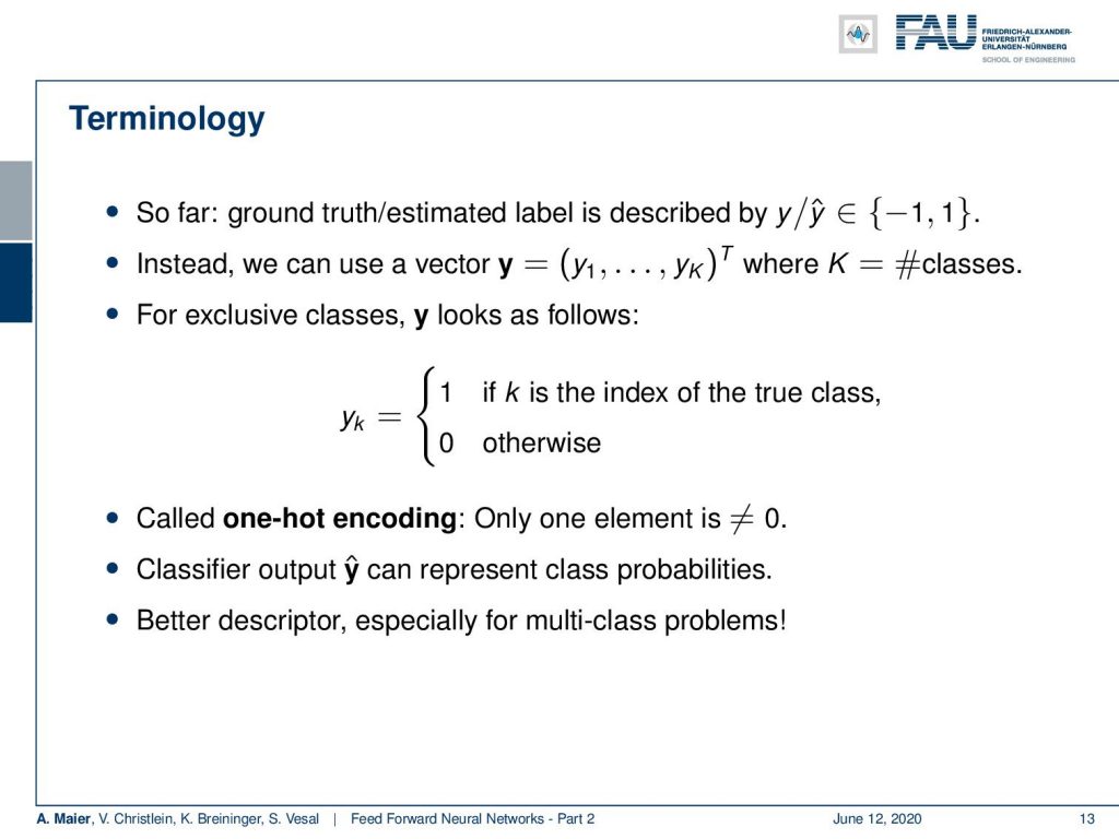
Now so far, we have described the ground truth by labels -1 and +1, but of course, we could also have classes 0 and 1. This is really only a matter of definition if we only do a decision between two classes. But if you want to go into more complex cases, you want to be able to classify multiple classes. So in this case, you probably want to have an output vector. Here, you have essentially one dimension per class k where K is the number of classes. You can then define a ground truth representation as a vector that has all zeros except for one position and that is the true class. So, this is also called one-hot encoding, because all of the other parts of the vector are 0. Only a single one has a 1. Now, you try to compute a classifier that will produce our respective vector, and with this vector y hat, you can then go ahead and do the classification.
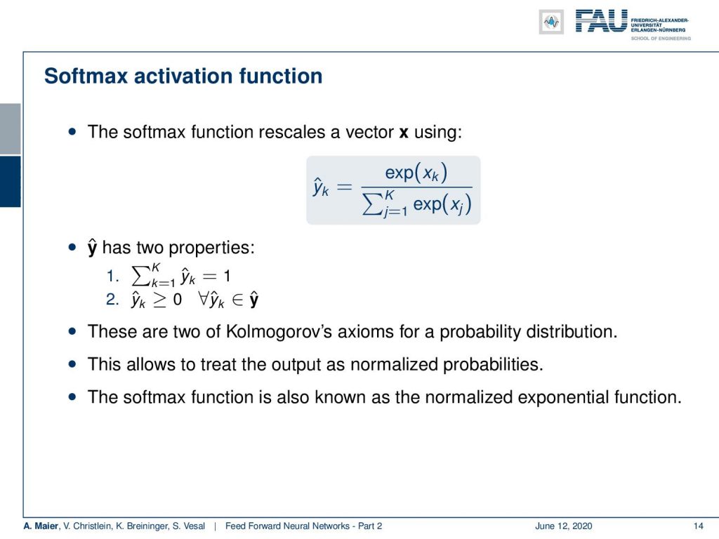
So it’s essentially like I’m guessing an output probability for each of the classes. In particular, for multi-class problems, this has been shown to be a more efficient way of attacking these problems. The problem is that you want to have a kind of probabilistic output towards 0 and 1, but we typically have some input vector x that could be arbitrarily scaled. So, in order to produce now our predictions, we employ a trick. The trick is that we use the exponential function as it will map everything into a positive space. Now, you want to make sure that the maximum that can be achieved is exactly 1. So, you do that for all of your classes and compute the sum over all of the exponentials of all input elements. This gives you the maximum that can be attained by this conversion. Then, you divide by this number for all of your given inputs and this will always scale to a [0, 1] domain. The resulting vector will also have the property that if you sum up all elements, it will equal to 1. These are two axioms of the probability distribution introduced by Kolmogorov. So, this allows us to treat the output of the network always as a kind of probability. If you look in literature also in software examples, sometimes the softmax function is also known as the normalized exponential function. It’s the same thing.
Now, let’s look at an example. So let’s say this is our input to our neural network. So, you see this small image on the left. Now, you introduce labels for this three-class problem. Wait, there’s something missing! It’s a four-class problem! So, you introduce labels for this four-class problem. Then, you have some arbitrary input that is shown here in the column x subscript k. So, they are scaled from -3.44 to 3.01. This is not so great, so let’s use the exponential function. Now, everything is mapped into positive numbers and there’s quite a difference now between the numbers. So, we need to rescale them and you can see that the highest probability is of course returned for heavy metal in this image!
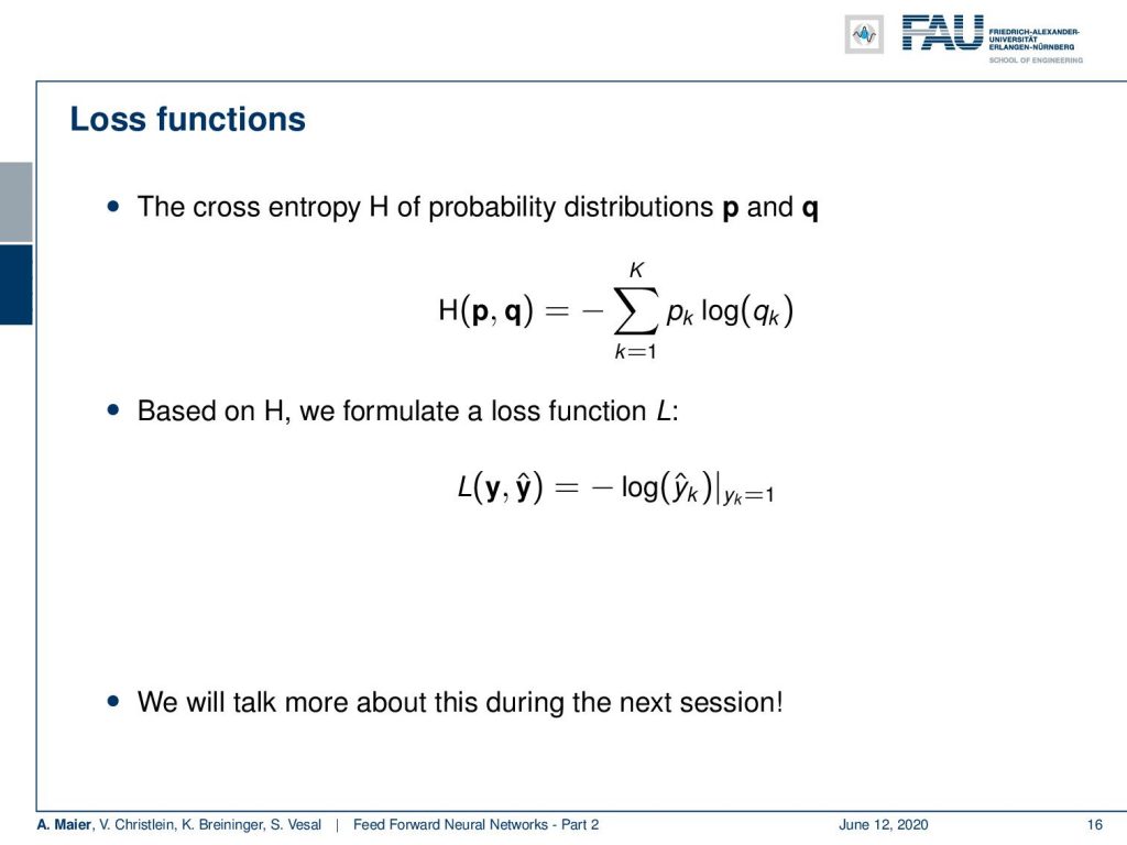
So, let’s go ahead and also talk a bit about loss functions. So the loss function is a kind of function that tells you how good the prediction of a network is. A very typical one is the so-called cross-entropy loss. The cross-entropy is computed between two probability distributions. So, you have your ground truth distribution and the one that you’re estimating. Then, you can compute the cross-entropy in order to determine how well they are connected, i.e. how well they align with each other. Then, you can also use this as a loss function. Here, we can use the property that all of our elements will be zero except for the true class. So we only have to determine the negative logarithm of y hat subscript k, where k is the true class. This simplifies the computation a lot and we get rid of the above sum. By the way, this has a couple of more interesting interpretations and we will talk about them in one of the next videos.
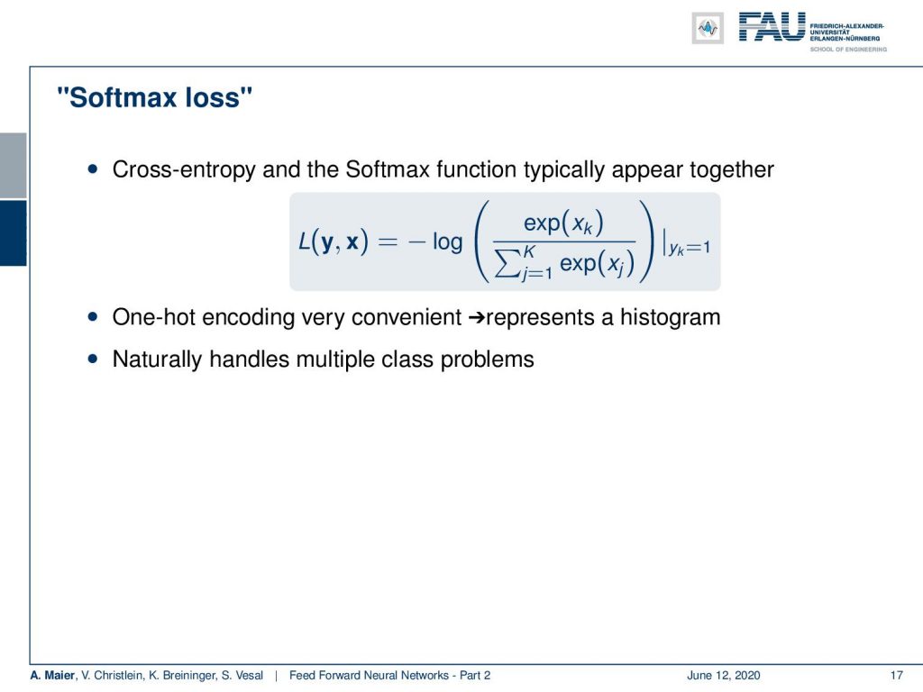
Now, if you do this we can plug in the softmax function and construct the so-called softmax loss. You can see, we have the softmax function in there and then we take minus logarithm only for the element that has the true class. This is something that very typically used in the training of networks. This softmax loss is very commonly used very useful for one hot encoded ground truth. Also, it kind of represents a histogram. It’s related to statistics and distributions. Furthermore, all of the multi-class problems can be handled in this approach in a single go.
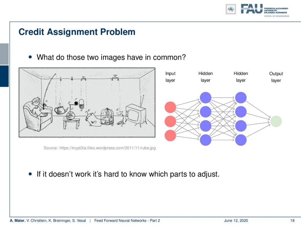
The other thing that I want to talk about in this video is optimization. So, one big thing that we haven’t considered at all is how we actually train those networks. We have already seen that these hidden layers that cannot be directly observed. This kind of brings us in a very difficult situation and you may argue that the image here on the right is very similar to the one on the left: If you change anything in this chain of events, it may essentially destroy the entire system. So, you have to be very careful in adjusting anything on the path, because you have to take into account all the other processing steps. This is really hard and you have to be careful what to adjust.
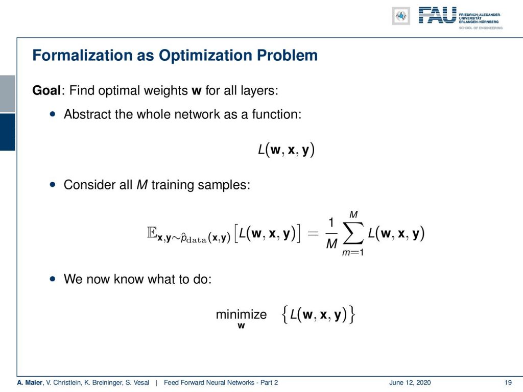
Now, we’ll go the easy way and we will formulate this as an optimization problem. So, we already discussed that we need some kind of loss function. The loss function tells us how good the fit of the predictions is to our actual training data. The inputs are the weights w, x the input vector, and y which are our ground truth labels. We have to consider all M training samples and this allows us to then describe some kind of loss. So, if we do this, we compute the expected value of the loss which is essentially the sum over all of the observations. This scaled sum then is used to determine the fit for the entire training data set. Now, if we want to create an optimal set of weights, what we do is we choose to minimize this loss function with respect to w over the entire training data set.
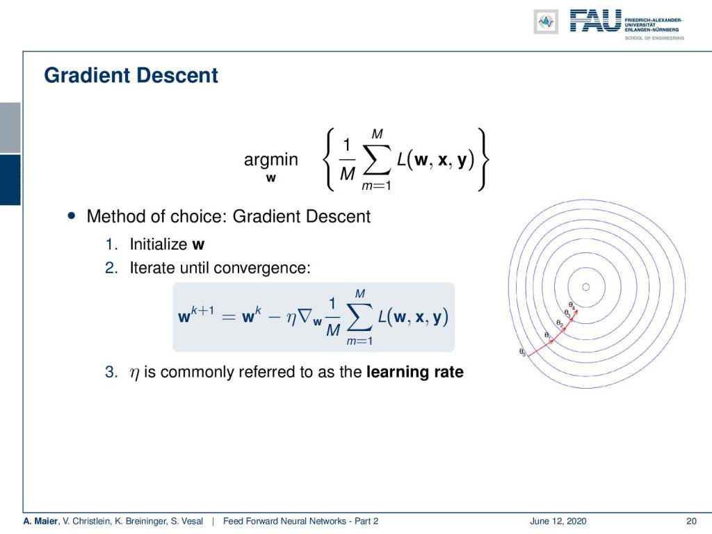
Well, now we have some mathematical principle that tells us what to do and we know minimization. Let’s try one of the obvious choices: gradient descent. So, we choose to find the minimum w that minimizes the loss of all training samples. In order to do so, we compute the gradient and we need some initial guess for w. There are many different ways of initializing w. Some people are just using randomly initialized weights and then you go ahead and do gradient descent. So, you follow the negative gradient direction step-by-step, until you arrive at some minimum. So here, you can see this initial w and this step may be random. Then in Step 2, iterate until convergence. So, you compute the gradient with respect to w of the loss function. Then you need some learning rate η. η essentially tells you how long the steps of these individual arrows here are. Then, you follow this direction until you arrive at a minimum. Now, η is commonly referred to as the learning rate. The interesting thing about this approach is it’s very simple and you will always find a minimum. It may be only a local one, but you will be able to minimize the function. What quite a few people do is they run several random initializations. Those random initializations are then used to find different local minima. Then, they simply take the best local minima for their final system.
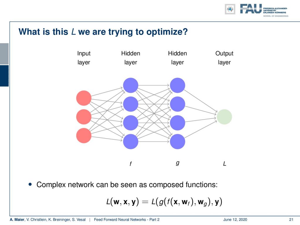
What is this L that we are trying to optimize? Well, L is computed here at the very output layer. So, we put in the input into our network process with the entire network, and then, in the end, we compute essentially the difference or the fit or the loss to our desired output. So you could say, if the first layer is f the second is g, then we are interested in computing L of some input x and w. We compute f using w subscript f. Then use the weights w subscript g, compute g and then, in the end, we compute the fit between g and y. So, this is essentially what we need to compute in the loss function.
You see that this is slightly more difficult and gets more difficult for deeper networks. So, we will see that we need to be able to do this efficiently. There’s a very efficient algorithm to solve such kind of problems and it’s called the backpropagation algorithm which will be the topic of our next lecture. So, thank you very much for listening and see you in the next video!
If you liked this post, you can find more essays here, more educational material on Machine Learning here, or have a look at our Deep Learning Lecture. I would also appreciate a clap or a follow on YouTube, Twitter, Facebook, or LinkedIn in case you want to be informed about more essays, videos, and research in the future. This article is released under the Creative Commons 4.0 Attribution License and can be reprinted and modified if referenced.
References
[1] R. O. Duda, P. E. Hart, and D. G. Stork. Pattern Classification. John Wiley and Sons, inc., 2000.
[2] Christopher M. Bishop. Pattern Recognition and Machine Learning (Information Science and Statistics). Secaucus, NJ, USA: Springer-Verlag New York, Inc., 2006.
[3] F. Rosenblatt. “The perceptron: A probabilistic model for information storage and organization in the brain.” In: Psychological Review 65.6 (1958), pp. 386–408.
[4] WS. McCulloch and W. Pitts. “A logical calculus of the ideas immanent in nervous activity.” In: Bulletin of mathematical biophysics 5 (1943), pp. 99–115.
[5] D. E. Rumelhart, G. E. Hinton, and R. J. Williams. “Learning representations by back-propagating errors.” In: Nature 323 (1986), pp. 533–536.
[6] Xavier Glorot, Antoine Bordes, and Yoshua Bengio. “Deep Sparse Rectifier Neural Networks”. In: Proceedings of the Fourteenth International Conference on Artificial Intelligence Vol. 15. 2011, pp. 315–323.
[7] William H. Press, Saul A. Teukolsky, William T. Vetterling, et al. Numerical Recipes 3rd Edition: The Art of Scientific Computing. 3rd ed. New York, NY, USA: Cambridge University Press, 2007.