Why do we need Deep Learning?
These are the lecture notes for FAU’s YouTube Lecture “Deep Learning“. This is a full transcript of the lecture video & matching slides. We hope, you enjoy this as much as the videos. Of course, this transcript was created with deep learning techniques largely automatically and only minor manual modifications were performed. If you spot mistakes, please let us know!
Welcome everybody to our lecture on deep learning! Today, we want to go into the topic. We want to introduce some of the important concepts and theories that have been fundamental to the field. Today’s topic will be feed-forward networks and feed-forward networks are essentially the main configuration of neural networks as we use them today. So in the next couple of videos, we want to talk about the first models and some ideas behind them. We also introduce a bit of theory. One important block will be about Universal function approximation where we will essentially show that neural networks are able to approximate any kind of function. This will then be followed by the introduction of the softmax function and some activations. In the end, we want to talk a bit about how to optimize such parameters and in particular, we will talk about the backpropagation algorithm.
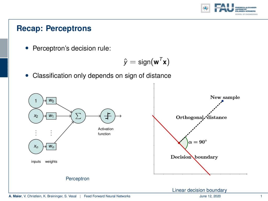
So let’s start with the model and what you heard already is the perceptron. We already talked about this which was essentially a function that would map any high dimensional input to an inner product of the weight vector and the input. Then, we are only interested in the signed distance that is computed. You can interpret this essentially as you see above on the right-hand side. The decision boundary is shown in red and what you’re computing with the inner product is essentially a signed distance of a new sample to this decision boundary. If we consider only the sign, we can decide whether we are on one side or the other.
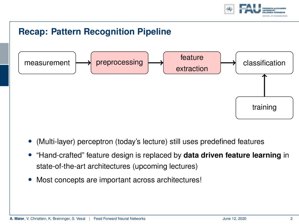
Now, if you look at classical pattern recognition and machine learning, we would still follow a so-called pattern recognition pipeline. We have some measurement that is converted and pre-processed in order to increase the quality, e.g. decrease noise. In the pre-processing, we essentially stay in the same domain as the input. So if you have an image as input, the output of the pre-processing will also be an image, but with probably better properties towards the classification task. Then, we want to do feature extraction. You remember the example with the apples and pears. From these, we extract features which then result in some high dimensional vector space. We can then go ahead and do the classification.
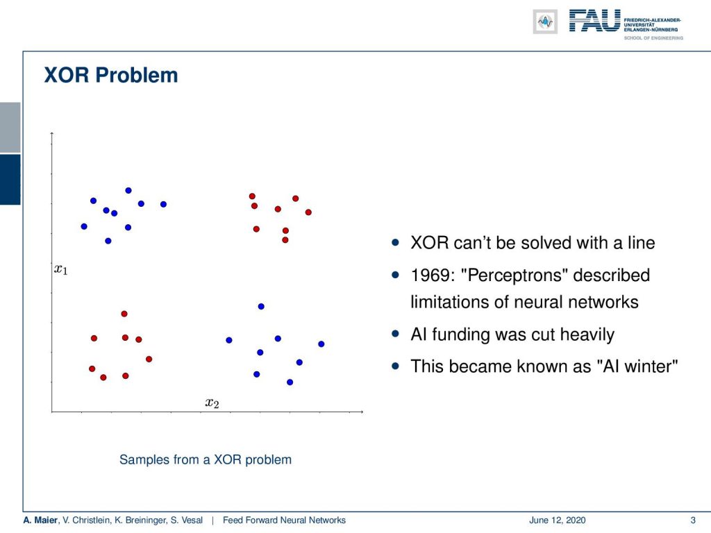
Now, what we’ve seen in the perceptron is that we are able to model linear decision boundaries. This immediately then led to the observation that perceptrons cannot solve the logical exclusive or – the so-called XOR. You can see the visualization of the XOR problem above on the left-hand side. So, imagine you have some kind of distribution of classes where the top left and the bottom right is blue and the other class is bottom left and top right. This is inspired by the logical XOR function. You will not be able to separate those two point clouds with a single linear decision boundary. So, you either need curves or you use multiple lines. With a single perceptron, you will not be able to solve this problem. Because people have been arguing: “Look we can model logical functions with perceptrons. If we build perceptrons on perceptrons, we can essentially build all of the logic!”

Now, if you can’t build XOR, then you’re probably not able to describe the entire logic and therefore, we will never achieve strong AI. This was a period of time when all funding to artificial intelligence research was tremendously cut down and people would not get any new grants. They would not get money to support the research. Hence, this period became known as the “AI Winter”.

Things changed with the introduction of the multi-layer perceptron. This is now the expansion of the perceptron. You do not just do a single neuron, but you use multiple of those neurons and you arrange them in layers. So here you can see a very simple draft. So, it is very similar to the perceptron. You have essentially some inputs and some weights. Now, you can see that it’s not just a single sum, but we have several of those sums that go through a non-linearity. Then, they assign weights again and summarize again to go into another non-linearity.
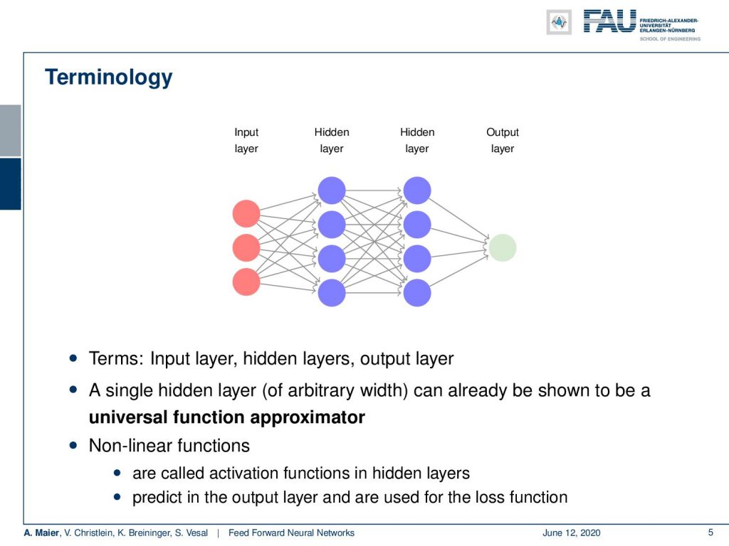
This is very interesting because we can use multiple neurons. We can now also model nonlinear decision boundaries. You can go on and then arrange this in layers. So what you typically do is, you have some input layer. This is our vector x. Then, you have several perceptrons that you arrange in hidden layers. They’re called hidden because they do not immediately observe the input. They assign weights, then compute something, and only at the very end, at the output, you have a layer again where you can observe what’s actually happening. All of these weights that are in between in those hidden layers, they are not directly observable. Here, you only observe them when you put some input in, compute the activations, and then at the very end, you can obtain the output. So, this is where you can actually observe what’s happening in your system.
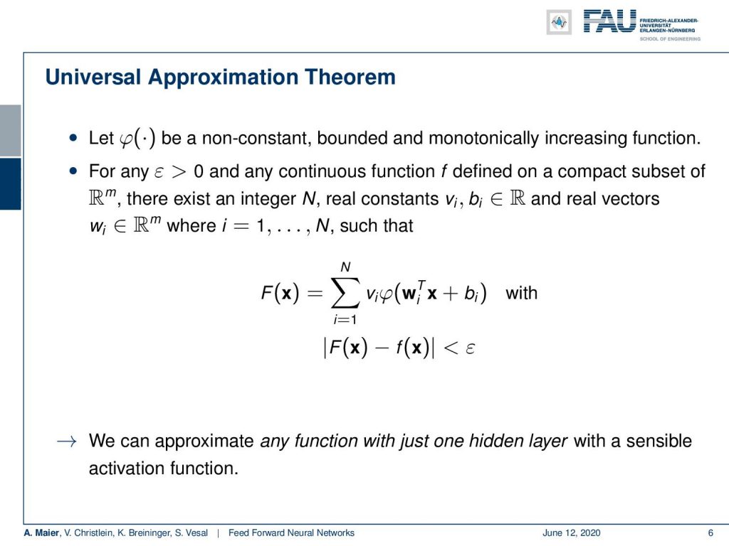
Now, we will look into the so-called universal function approximator. This is actually just a network with a single hidden layer. Universal function approximation is a fundamental piece of theory because it tells us that with a single hidden layer, we can approximate any continuous function.
So, let’s look a bit into this theorem. It starts as a formal definition. We have some 𝜑(x) and 𝜑(x) is a non-constant, bounded, monotonically increasing function. There exists some 𝜀 greater than zero and for any continuous function f(x) defined on a compact subset of some high dimensional space ℝᵐ there exists an integer and real constant 𝜈 and b, and the real vectors w, where you can find an approximation. Here, you now see how the approximation is computed. You have an inner product of the weights with the input plus some bias. This goes into some activation function 𝜑(x). This is a non-constant, bounded, and monotonically increasing function. Then you have another linear combination using those 𝜈 which then produce the output capital F(x). So F(x) is our approximation and the approximation is a linear combination of nonlinearities that are computed from linear combinations. If you define it this way, you can demonstrate that if you F(x) from the true function f(x), the absolute difference between the two is bounded by a constant 𝜀. 𝜀 is greater than zero.

That’s already a very useful approximation. There is an upper bound 𝜀, but right now it doesn’t tell us how large 𝜀 actually is. So, 𝜀 may be really large. The universal approximation theorem also tells us that if we increase N, then 𝜀 goes down. Now if you approach infinity with N, 𝜀 will approach zero. So, the more neurons we take in this hidden layer, the better our approximation will get. So this means, we can approximate any function with just one hidden layer. So you could argue if you can approximate everything with a single layer, why the hell are people doing deep learning?
Deep learning doesn’t make any sense if a single layer is enough. I’ve just proved this to you. So there’s maybe no need for deep learning? Let’s look into some examples: I took a classification tree here and a classification tree is a method of subdividing space. I’m taking a 2-D example here where we have some input space x₁ and x₂. This is useful because we can visualize it very efficiently here on the slides. Our decision tree does the following thing: It decides whether x₁ is greater than 0.5. Note that I’m showing you the decision boundary on the right. In the next node, if you go to the left-hand side you look at x₂ and decide whether it’s greater or smaller than 0.25. On the other side, you simply look at x₁ again and decide whether it’s greater or smaller than 0.75. Now, if you do that you can assign classes in the leaf nodes. In these leaves, you can now, for example, assign the value 0 or 1 and this gives a subdivision of this place that has the shape of a mirrored L.
So, this is a function and this function can now be approximated by a universal function approximator. So let’s try to do that. We can transform this actually into a network. Let’s use the following idea: Our network has 2 input neurons because it’s a two-dimensional space. With our decision boundaries, we can also form these decisions x₁ being greater or smaller than 0.5. So, we can immediately adopt this. We can actually also adopt all the other inner nodes. Because we are using a sigmoid in this example, we also use the inverse of the inner nodes and put them in as additional neurons. So of course, I don’t have to learn anything here, because the connections towards the first hidden layer, I can take them from the tree definition. They’re already predefined, so there’s no learning required here. On the output side, I have to learn some weights and this can be done using for example a least square approximation and then I can directly compute those weights.
If I go ahead and really do that, we can also find a nice visualization. You can see that with our decision boundaries, we are essentially constructing a basis in the hidden layer. You can see if I use 0 and 1 as black and white, for every hidden node, I’m constructing a base vector. They are then essentially weighted linearly to for the output. So you could do this here by multiplying every pixel with every pixel and then simply summing this up. This is what the hidden layer here would do. Then, I’m essentially interested in combining those space vectors such that it will produce the desired y. Now, if I do that in a least-square sense, I get the approximation on the right. So it’s not half bad. I magnified this a bit. So this is what we wanted to get. This is the mirrored L and this is what came out of my approximation that I just proposed. Now, you can see that it kind of has the L shape in there, but the values here are in a domain between [0,1] and the 𝜀 with my six neuron approximation here is probably in the range of 0.7. So it kind of does the trick, but the approximation is not very good. In this particular configuration, you have to increase the number of neurons really a lot in order to get the error down because it’s a really hard problem. It can almost not be approximated.
So, what else could we do? Well if we want this, we could for example add a second non-linearity. Then, we would get exactly the solution that we desire. So you see maybe one layer is not very efficient in terms of representation. There is an algorithm that can map any decision tree on to a neural network. The algorithm goes as follows: You take all of your inner nodes, here the decisions between 0.5, 0.25, and 0.75. So, these are the inner nodes and then you connect them appropriately. You connect them in a way such that you are able to form exactly the sub-regions. Here you see that this is our L shape and in order to construct the top left region, we need to have access to the first decision. It separates the space into the left half-space and the right-half space. Next, we have access to the second decision. This way, we can use these two decisions in order to form this small patch on the top left. For all of the four patches that emerge from the decision boundaries, we get essentially one node. This simply means that for every leaf node, we get one node in the second layer. So one node for every inner node in the first layer and one node for every leaf node in the second layer. Then, you combine them in the output. You don’t even have to compute anything here, because we already know how these have to be merged in order to get to the right decision boundaries. This way, we manage to convert your decision tree into a neural network and it does exactly the correct approximation as we want it to happen.
What do we learn from this example? Well, we can approximate any function with a universal function approximator with just one hidden layer. But if we go deeper, we may find a decomposition of the problem that is just way more efficient. So here the decomposition was first inner nodes, then leaf nodes. This enabled us to derive an algorithm that only has seven nodes and could exactly approximate the problem. So you could argue that by building deeper networks you add additional steps. In each step, you try to simplify the function and the power of the representation, such that you get better processing towards the decision in the end.
Now, let’s go back to our Universal function approximation theorem. So, we’ve seen that it exists. It tells us that we can approximate everything with just a single hidden layer. So, that’s already a pretty cool observation but it doesn’t tell us how to choose N. It doesn’t tell us how to train. So there are a lot of problems with the universal approximation theorem. This is essentially the reason, why we go to what’s deep learning. Then, we can build systems that start disentangling representation over various steps. If we do so, we can build more efficient and more powerful systems and train them end-to-end. So this is the main reason, why we go towards deep learning. I expect anybody who’s working in deep learning to know about universal approximation and why deep learning actually makes sense. Ok so, that’s it for today. Next time, we will talk about activation functions and we will start introducing the backpropagation algorithm in the next set of videos. So stay tuned! I hope you enjoyed this video. Looking forward to seeing you in the next one!
If you liked this post, you can find more essays here, more educational material on Machine Learning here, or have a look at our Deep Learning Lecture. I would also appreciate a clap or a follow on YouTube, Twitter, Facebook, or LinkedIn in case you want to be informed about more essays, videos, and research in the future. This article is released under the Creative Commons 4.0 Attribution License and can be reprinted and modified if referenced.
References
[1] R. O. Duda, P. E. Hart, and D. G. Stork. Pattern Classification. John Wiley and Sons, inc., 2000.
[2] Christopher M. Bishop. Pattern Recognition and Machine Learning (Information Science and Statistics). Secaucus, NJ, USA: Springer-Verlag New York, Inc., 2006.
[3] F. Rosenblatt. “The perceptron: A probabilistic model for information storage and organization in the brain.” In: Psychological Review 65.6 (1958), pp. 386–408.
[4] WS. McCulloch and W. Pitts. “A logical calculus of the ideas immanent in nervous activity.” In: Bulletin of mathematical biophysics 5 (1943), pp. 99–115.
[5] D. E. Rumelhart, G. E. Hinton, and R. J. Williams. “Learning representations by back-propagating errors.” In: Nature 323 (1986), pp. 533–536.
[6] Xavier Glorot, Antoine Bordes, and Yoshua Bengio. “Deep Sparse Rectifier Neural Networks”. In: Proceedings of the Fourteenth International Conference on Artificial Intelligence Vol. 15. 2011, pp. 315–323.
[7] William H. Press, Saul A. Teukolsky, William T. Vetterling, et al. Numerical Recipes 3rd Edition: The Art of Scientific Computing. 3rd ed. New York, NY, USA: Cambridge University Press, 2007.