
Performance Evaluation
These are the lecture notes for FAU’s YouTube Lecture “Deep Learning“. This is a full transcript of the lecture video & matching slides. We hope, you enjoy this as much as the videos. Of course, this transcript was created with deep learning techniques largely automatically and only minor manual modifications were performed. If you spot mistakes, please let us know!
Welcome everybody to the next part of deep learning! Today, we want to finish talking about common practices, and in particular, we want to have a look at the evaluation. Of course, we need to evaluate the performance of the models that we’ve trained so far. Now, we have set up the training, set hyperparameters, and configured all of this. Now, we want to evaluate the generalization performance on previously unseen data. This means the test data and it’s time to open the vault.
Remember “Of all things the measure is man”. So, data is annotated and labeled by humans and during training, all labels are assumed to be correct. But of course, to err is human. This means we may have ambiguous data. The ideal situation that you actually want to have for your data is that it has been annotated by multiple human voters. Then you can take the mean or a majority vote. There’s also a very nice paper by Stefan Steidl from 2005. It introduces an entropy-based measure that takes into account the confusions of human reference labelers. This is very useful in situations where you have unclear labels. In particular, in emotion recognition, this is a problem as also humans confuse sometimes classes like angry versus annoyed while they are not very likely to confuse “angry” versus “happy” as this is a very clear distinction. There are different degrees of happiness. Sometimes you’re just a little bit happy. In these cases, it is really difficult to differentiate happy from neutral. This is also hard for humans. In prototypes, if you have for example actors playing, you get emotion recognition rates way over 90%. If you have real data emotion and if you have emotions as they occur in daily life, it’s much harder to predict. This can then also be seen in the labels and in the distribution of the labels. If you have a prototype, all of the raters will agree that the observation is clearly this particular class. If you have nuances and not so clear emotions, you will see that also our raters will have a less peaked or even a uniform distribution over the labels because they also can’t assess the specific sample. So, mistakes by the classifier are obviously less severe if the same class is also confused by humans. Exactly this is considered in Steidl’s entropy-based measure.
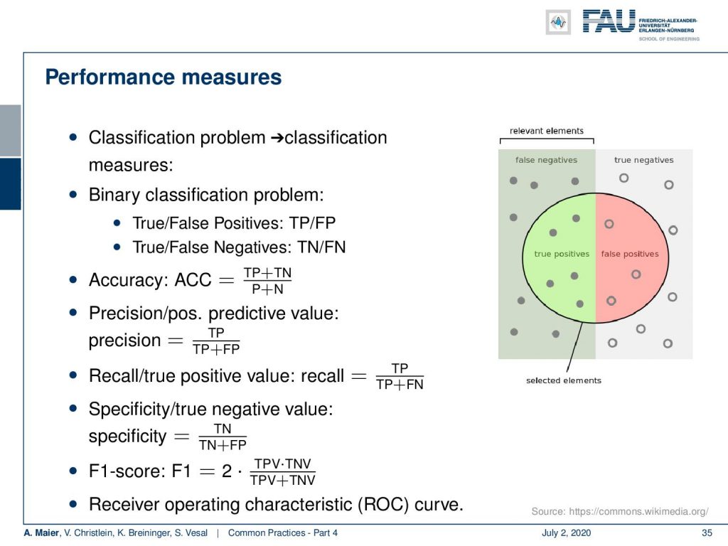
Now, if we look into performance measures, you want to take into account the typical classification measures. They are typically built around the false negatives, the true negatives, the true positives, and the false positives. From that for binary classification problems, you can then compute true and false positive rates. This typically then leads to numbers like the accuracy that is the number of true positives plus true negatives over the number of positives and negatives. Then, there is the precision or positive predictive value that is computed as the number of true positives over the number of true positives plus false positives. There’s the so-called recall that is defined as the true positives over the true positives plus the false negatives. Specificity or true negative value is given as the true negatives over the true negatives plus the false positives. The F1 score is an intermediate way of mixing these measures. You have the true positive value times the true negative value divided over the sum of two positive and true negative value. I typically recommend the receiver operating characteristic (ROC) curves because all of the measures that you’ve seen above, they are dependent on thresholds. If you have the ROC curves, you essentially evaluate your classifier for all different thresholds. This then gives you an analysis of how well it performs in different scenarios.
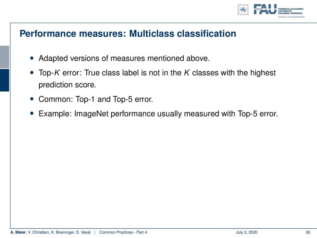
Furthermore, there are performance measures in multi-class classification. These are adapted versions of the measures above. The top-K error is the probability of the true class label not being in the K estimates with the highest prediction score. Common realizations are the top-1 and top-5 error. ImageNet, for example, usually uses the top-5 error. If you really want to understand what’s going on in multi-class classification, I recommend looking at confusion matrices. Confusion matrices are useful for let’s say 10 to 15 classes. If you have a thousand classes, confusion matrices don’t make any sense anymore. Still, you can gain a lot of understanding of what’s happening if you look at confusion matrices in cases with fewer classes.
Now, sometimes you have very few data. So, in these cases, you may want to choose cross-validation. In k-fold cross-validation, you split your data into k folds, and then you use k – 1 folds as training data and test on Fold k. Then, you repeat it k times. This way, you have seen in the evaluation data all of the data but you trained on independent data because you held it out at the time of training. It’s rather uncommon in deep learning because it implies very long training times. You have to repeat the entire training K times which is really hard if you train for like seven days. If you have sevenfold cross-validation, you know you can do the math, it will take really long. If you use it for hyperparameter estimation, you have to nest it. Don’t perform cross-validation just on all of your data, select the hyperparameters, and then go ahead with the same data in testing. This will give you optimistic results. You should always make sure that if you select parameters you hold out the test data where you want to test on so there’s techniques for nesting cross-validation into cross-validation but then it will also become computationally very expensive so that’s even worse if you want to nest the cross-validation one thing that you have to keep in mind is that the variance of the results is typically underestimated because the training grants are not independent also pay attention that you may introduce additional bias by incorporating the architecture selection and hyperparameter selection so this should be done on different data and it’s very difficult if you’re working with cross-validation even without cross-validation training is a highly stochastic process therefore you may want to retrain your network multiple times with different initializations if you pick random initializations for example and then report the standard deviation just to make sure how well your training actually performs.
Now, you want to compare different classifiers. The question is: “Is my new method with 91.5% accuracy better than the state-of-the-art with 90.9%?” Of course, training a system is a stochastic process. So, just comparing those two numbers will yield biased results. The actual question that you have to ask is: “Is there a significant difference between the classifiers?” This means that you need to run the training for each method multiple times. Only then you can, for example, use a t-test to see whether the distribution of the results is significantly different. The t-test compares two normally distributed data sets with equal variance. Then, you can determine that the means are significantly different with respect to a significance level α which is the level of randomness. Quite frequently you find in literature like 5% or 1% significance level. So you have a significant difference if the chance of this observation being random is less than 5% or 1%.
Now be careful if you train multiple models on the same data. If you ask the same data a couple of times, you actually have to correct your significance computation. This is called the Bonferroni correction. If we compare multiple classifiers, this will introduce multiple comparisons and then you have to correct for this. If you had n tests with significance level α, then the total risk is n times α. So, to reach the total significance level of α, the adjusted α’ would be α over n for each individual test. So, the more tests you run on the same data, the more you have to divide by. Of course, this assumes independence between the tests and it’s a kind of pessimistic estimation of significance. But you want to be pessimistic in this case just to make sure that you are not reporting something that has been produced by chance. Just because you test often enough and your testing is a random process, there may be a very good result showing up just by chance. More accurate, but incredibly time-consuming would be permutation tests, and believe me, you probably want to go with the Bonferroni correction instead. Permuting everything will take even longer than the cross-validation approach that we’ve seen previously.
Okay so let’s summarize what we’ve seen before: You check your implementation before training, the gradient initialization, monitor the training process continuously, the training, the validation losses, the weights, and the activations. Stick to established architectures before reinventing the wheel. Experiment with little data and keep your evaluation data safe until the evaluation. Decay the learning rate over time. Do a random search, not a grid search for hyperparameters. Perform model ensembling for better performance, and when you check your comparison, of course, you want to go for significance tests to make sure that you are not reporting a random observation.
So next time on deep learning, we actually want to look at the evolution of neural network architectures. So from deep networks to even deeper networks. We want to have a look at sparse and dense connections and we’ll introduce a lot of common names, things you hear all over the place, LeNet, GoogLeNet, ResNet, and so on. So we will learn about many interesting state-of-the-art approaches in this next series of lecture videos. So, thank you very much for listening and see you in the next video!
If you liked this post, you can find more essays here, more educational material on Machine Learning here, or have a look at our Deep LearningLecture. I would also appreciate a follow on YouTube, Twitter, Facebook, or LinkedIn in case you want to be informed about more essays, videos, and research in the future. This article is released under the Creative Commons 4.0 Attribution License and can be reprinted and modified if referenced.
Links
References
[1] M. Aubreville, M. Krappmann, C. Bertram, et al. “A Guided Spatial Transformer Network for Histology Cell Differentiation”. In: ArXiv e-prints (July 2017). arXiv: 1707.08525 [cs.CV].
[2] James Bergstra and Yoshua Bengio. “Random Search for Hyper-parameter Optimization”. In: J. Mach. Learn. Res. 13 (Feb. 2012), pp. 281–305.
[3] Jean Dickinson Gibbons and Subhabrata Chakraborti. “Nonparametric statistical inference”. In: International encyclopedia of statistical science. Springer, 2011, pp. 977–979.
[4] Yoshua Bengio. “Practical recommendations for gradient-based training of deep architectures”. In: Neural networks: Tricks of the trade. Springer, 2012, pp. 437–478.
[5] Chiyuan Zhang, Samy Bengio, Moritz Hardt, et al. “Understanding deep learning requires rethinking generalization”. In: arXiv preprint arXiv:1611.03530 (2016).
[6] Boris T Polyak and Anatoli B Juditsky. “Acceleration of stochastic approximation by averaging”. In: SIAM Journal on Control and Optimization 30.4 (1992), pp. 838–855.
[7] Prajit Ramachandran, Barret Zoph, and Quoc V. Le. “Searching for Activation Functions”. In: CoRR abs/1710.05941 (2017). arXiv: 1710.05941.
[8] Stefan Steidl, Michael Levit, Anton Batliner, et al. “Of All Things the Measure is Man: Automatic Classification of Emotions and Inter-labeler Consistency”. In: Proc. of ICASSP. IEEE – Institute of Electrical and Electronics Engineers, Mar. 2005.