
Hyperparameters and Ensembling
These are the lecture notes for FAU’s YouTube Lecture “Deep Learning“. This is a full transcript of the lecture video & matching slides. We hope, you enjoy this as much as the videos. Of course, this transcript was created with deep learning techniques largely automatically and only minor manual modifications were performed. If you spot mistakes, please let us know!
Welcome everybody to deep learning! So, today we want to look into further common practices and in particular, in this video, we want to discuss architecture selection and hyperparameter optimization.
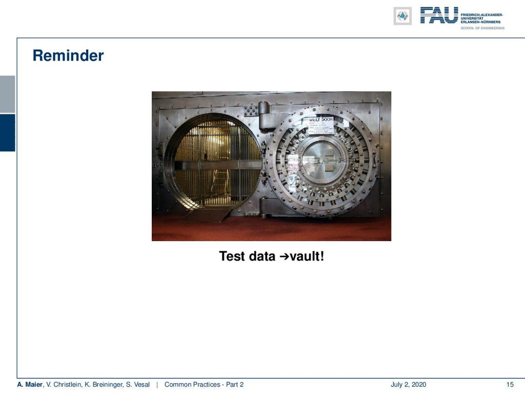
Remember the test data is still in the vault. We are not touching it. However, we need to set our hyperparameters somehow and you’ve already seen that there’s an enormous amount of hyperparameters.
You have to select an architecture, a number of layers, number of nodes per layer, activation functions, and then you have all the parameters in the optimization: the initialization, the loss function, and many more. The optimizers still have options like the type of gradient descent, momentum, learning rate decay, and batch size. In regularization, you have different regularizes L2 and L1 loss, batch normalization, dropout, and so on. You want to somehow figure out all the parameters for those different kinds of procedures.
Now, let’s choose an architecture and loss function. The first step would be to think about the problem and the data. How could features look like? What kind of spatial correlation do you expect? What data augmentation makes sense? How will the classes be distributed? What is important regarding the target application? Then you start with simple architectures and loss functions and of course, you do your research. Try well-known models first and foremost. They are being published and there are so many papers out there. Hence, there is no need to do everything yourself. One day in the library can save hours, weeks, and months of experimentation. Do the research. It will really save you time. Often they just don’t publish the paper, but in very good papers, it’s not just the scientific result, but they also share source code, Sometimes even data. Try to find those papers. This can help you a lot with your own experimentation. So, then you may want to change and adapt the architecture to your problem that you found in the literature. If you change something, find good reasons why this is an appropriate change. There are quite a few papers out there that seem to introduce random changes into the architecture. Later, it turns out that the observations that they made were essentially random and they were just lucky or experimented enough on their own data in order to get the improvements. Typically, there’s also a reasonable argument of why the specific change should give an improvement in performance.
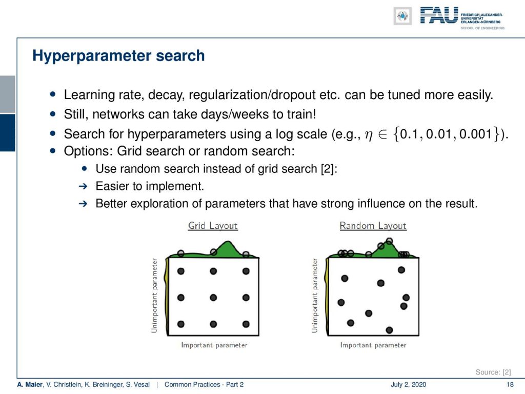
Next, you want to do your hyperparameter search. So you remember learning rate decay, regularization, dropout, and so on. These have to be tuned. Still, the networks can take days or weeks to train and you have to search for these hyperparameters. Hence, we recommend using a log scale. So, for example for η here you go for 0.1, 0.01, and 0.001. You may want to consider a grid search or random search. So in a grid search, you would have equal distance steps and if you look here at reference [2], they have shown that random search has advantages over the grid search. First of all, it’s easier to implement, and second, it has a better exploration of the parameters that have a strong influence. So, you may want to look into that and then adjust your strategy accordingly. So hyperparameters are highly interdependent. You may want to use a coarse to fine search. You optimize on a very coarse scale in the beginning and then make it finer. You may only train the network for a few epochs and then bring all the hyperparameters in sensible ranges. Then, you can refine using random and grid search.
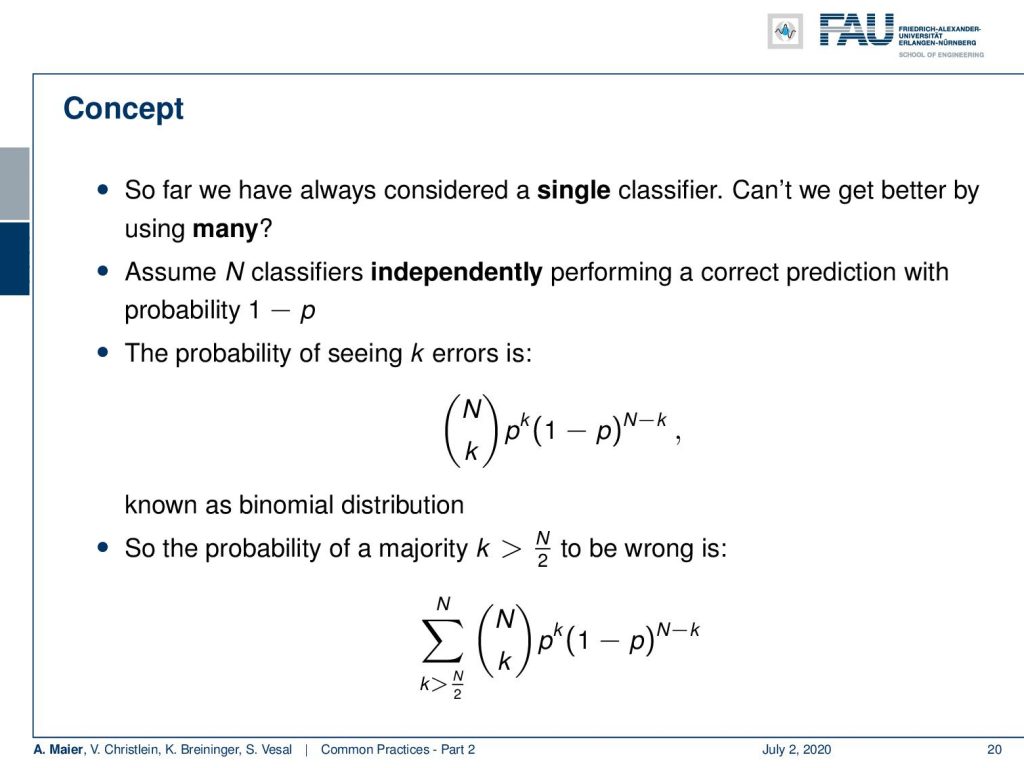
A very common technique that can give you a little bit of boost of performance is ensembling. This is also something that can really help you to get this additional little bit of performance that you still need. So far, we have only considered a single classifier. Ensembling has the idea to use many of those classifiers. If we assume N classifiers that are independent, performing a correct prediction will be at a probability of 1 – p. Now, the probability of seeing k errors is N choose k times p to the power of k times (1 – p) to the power of (N – k). This is a binomial distribution. So, the probability of a majority meaning k > N/2 to be wrong is the sum over N choose k times p to the power of k times (1 – p) to the power of (N – k).
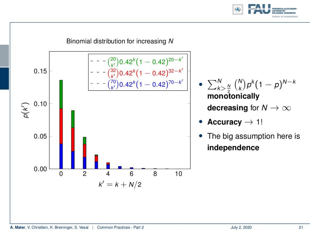
So, we visualize this in the following plot here. In this graph, you can see that if I take more of those weak classifiers, we get stronger. Let’s set for example their probability of being wrong to 0.42. Now, we can compute this binomial distribution. Here, you can see that if I choose 20, I get a probability of approximately 14% that the majority is wrong. If I choose N=32, I get less than 10% probability that the majority is wrong. If I choose 70, more than 95% of the cases the majority will be correct. So, you see that this probability is monotonically decreasing for large N. If n approaches infinity, then the accuracy will go towards 1. The big problem here is, of course, independence. So typically, we have problems generating from the same data, independent classifiers. So, if we had of course enough data then we can train many of those independent weak classifiers. So, how do we then implement this as a concept? We somehow have to produce N independent classifiers or regressors and then we combine the predictions by majority or averaging. How can we actually produce such components?
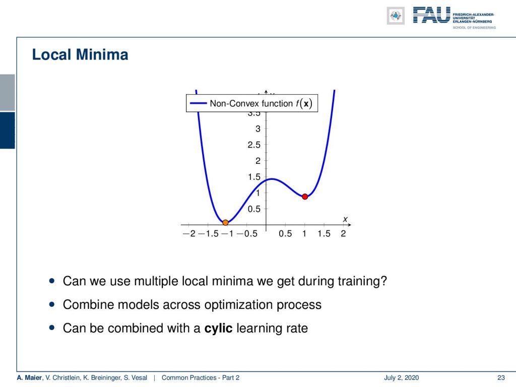
Well, you can choose different models. So in the example here, we have seen that we have a non-convex function. Obviously, they have different local minima. So, the different local minima would result in different models and then we can combine them. Also, what you can try is a cyclic learning rate where you then go up and down with the learning rate to escape certain local minima. This way, you can then try to find different local minima and store them for ensembling.
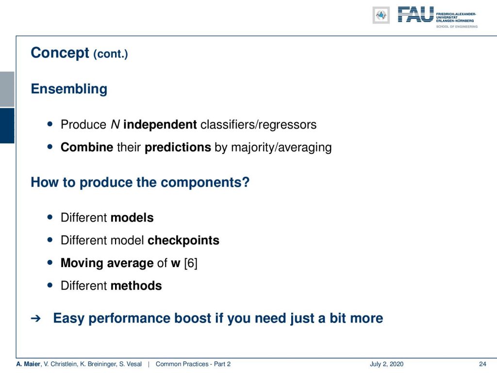
This way, you could also take different model checkpoints that you extract at different points in the optimization. Later, you can reuse them for ensembling. Also, a moving average of weights w can generate new models. You could even go this far and combine different methods. So, we still have the entire catalog of traditional machine learning approaches that you could also train and then combine them with your new deep learning model. Typically, this is an easy boost of performance if you need just a little bit more. By the way, this was also the idea that finally helped people to break the Netflix challenge. The first two teams that almost broke the challenge, they teamed up and trained an ensemble. This way they broke the challenge together.
So next time in deep learning, we will talk about class imbalance, a very frequent problem, and how to deal with that in your training procedure. Thank you very much for listening and goodbye!
If you liked this post, you can find more essays here, more educational material on Machine Learning here, or have a look at our Deep LearningLecture. I would also appreciate a follow on YouTube, Twitter, Facebook, or LinkedIn in case you want to be informed about more essays, videos, and research in the future. This article is released under the Creative Commons 4.0 Attribution License and can be reprinted and modified if referenced.
References
[1] M. Aubreville, M. Krappmann, C. Bertram, et al. “A Guided Spatial Transformer Network for Histology Cell Differentiation”. In: ArXiv e-prints (July 2017). arXiv: 1707.08525 [cs.CV].
[2] James Bergstra and Yoshua Bengio. “Random Search for Hyper-parameter Optimization”. In: J. Mach. Learn. Res. 13 (Feb. 2012), pp. 281–305.
[3] Jean Dickinson Gibbons and Subhabrata Chakraborti. “Nonparametric statistical inference”. In: International encyclopedia of statistical science. Springer, 2011, pp. 977–979.
[4] Yoshua Bengio. “Practical recommendations for gradient-based training of deep architectures”. In: Neural networks: Tricks of the trade. Springer, 2012, pp. 437–478.
[5] Chiyuan Zhang, Samy Bengio, Moritz Hardt, et al. “Understanding deep learning requires rethinking generalization”. In: arXiv preprint arXiv:1611.03530 (2016).
[6] Boris T Polyak and Anatoli B Juditsky. “Acceleration of stochastic approximation by averaging”. In: SIAM Journal on Control and Optimization 30.4 (1992), pp. 838–855.
[7] Prajit Ramachandran, Barret Zoph, and Quoc V. Le. “Searching for Activation Functions”. In: CoRR abs/1710.05941 (2017). arXiv: 1710.05941.
[8] Stefan Steidl, Michael Levit, Anton Batliner, et al. “Of All Things the Measure is Man: Automatic Classification of Emotions and Inter-labeler Consistency”. In: Proc. of ICASSP. IEEE – Institute of Electrical and Electronics Engineers, Mar. 2005.