The Rise of the Residual Connections
These are the lecture notes for FAU’s YouTube Lecture “Deep Learning“. This is a full transcript of the lecture video & matching slides. We hope, you enjoy this as much as the videos. Of course, this transcript was created with deep learning techniques largely automatically and only minor manual modifications were performed. If you spot mistakes, please let us know!
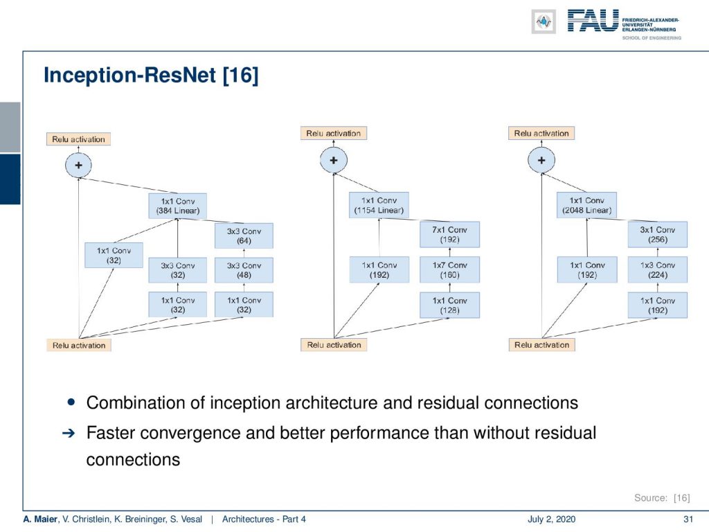
Welcome back to deep learning! As promised in the last video, we want to go ahead and talk a bit about more sophisticated architectures than the residual networks that we’ve seen in the previous video. okay, what do I have for you? Well, of course, we can use this recipe of the residual connections also with our inception network, and then this leads to inception ResNet. You see that the idea of residual connections is so easy that you can very easily incorporate it into many of the other architectures. This is also why we present these couple of architectures here. They are important building blocks towards building really deep networks.
You can see here that the inception and ResNet architectures really help you also to build very powerful networks. I really like this plot because you can learn a lot from it. So, you see on the y-axis, the performance in terms of top one accuracy. You see on the x-axis the number of operations. So, this is measured in gigaflops. Also, you see the number of parameters of the models indicated by the diameter of the circle. Here, you can see that VGG-16 and VGG-19, they’re at the very far right. So, they’re very computationally expensive and their performance is kind of good, but not as good as other models that we’ve seen here in this class. You also see that AlexNet is on the bottom left. So it doesn’t have too many computations. Also, in terms of parameters, it’s quite a bit large but the performance is not too great. Now, you see if you do batch normalization and network-in-network, you get better. Then there are the GoogleNet and ResNet-18 that have an increased top one accuracy. We see that we can now go ahead to build deeper models, but not get too many new parameters. This helps us to build more effective and more performing networks. Of course, then after some time, we also start increasing the parameter space and you can see that the best performances are here obtained with inception V3 or inception V4 networks or also Resnet-100.
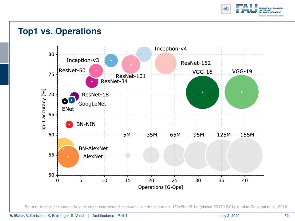
Well, what are other recipes that can help you build better models? One thing that we’ve seen quite successfully is increasing the width of the residual networks. So, there are wide residual networks. They decrease the depth but they increase the width of the residual blocks. Then, you also use dropout in these residual blocks and you can show that a 16-layer deep network with a similar number of parameters can outperform a thousand-layer deep network. So here, the power is not from depth but from the residual connections and the width that’s introduced.
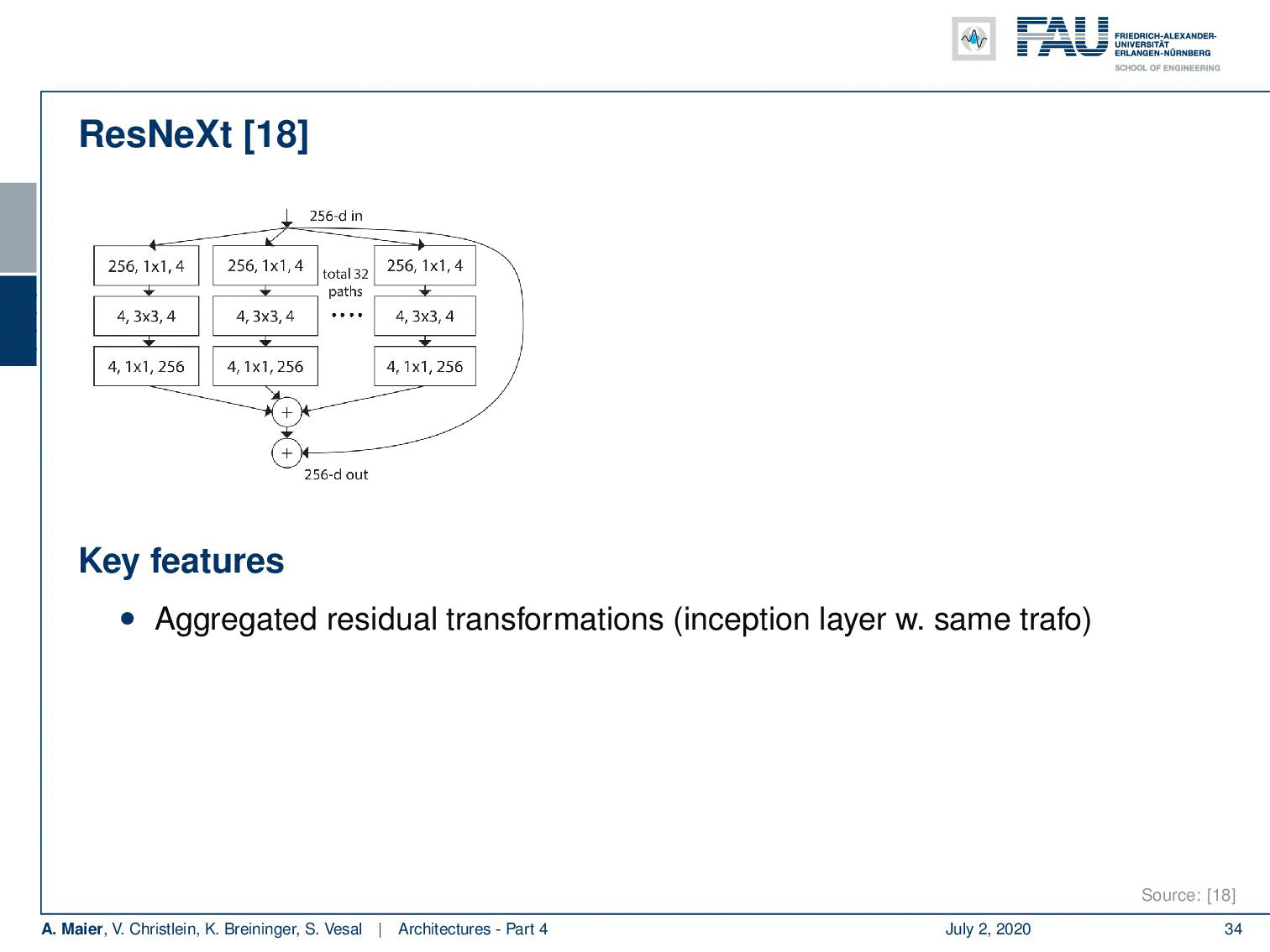
There are also things like ResNeXt, where all of the previous recipes have been built together. It allows aggregated residual transformations. So, you can see that this is actually equivalent to early concatenation. So, we can replace it with early concatenation and then the general idea is that you do group convolution. So, you have the input and output chains divided into groups and then the convolutions are performed separately within every group. Now, this has similar flops and number of parameters as a ResNet bottleneck block, but it’s wider and a sparsely connected module. So this is quite popular.
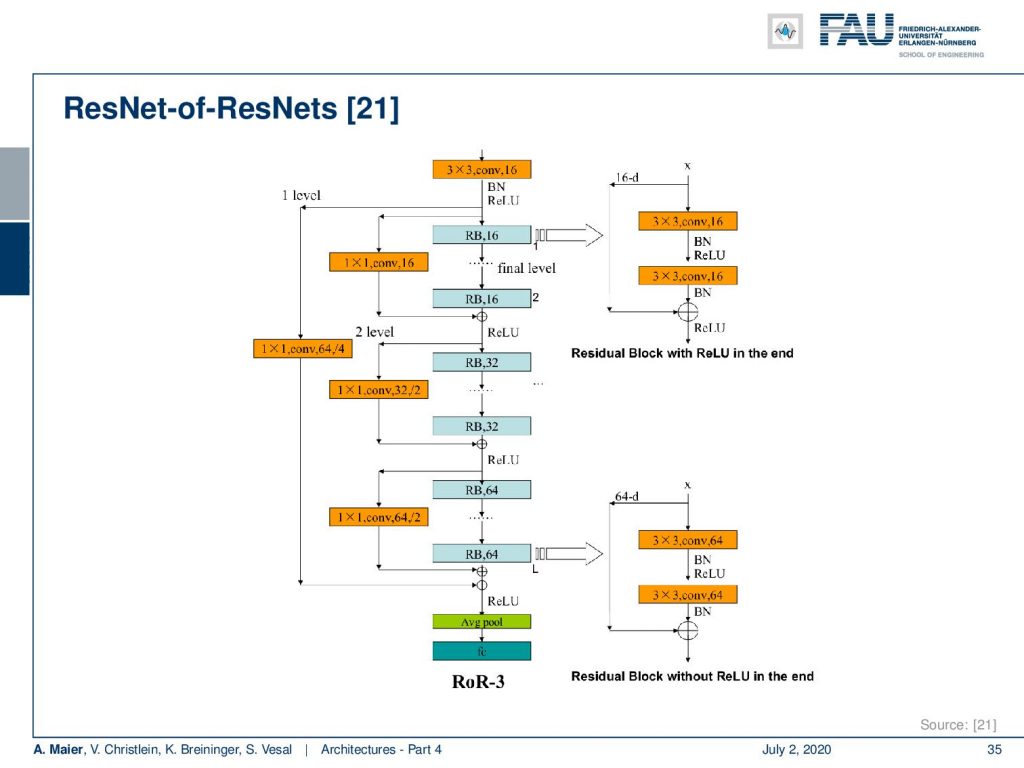
Then, of course, you can combine this with other ideas. In ResNet-of-ResNets, you can even build more residual connections into the network.
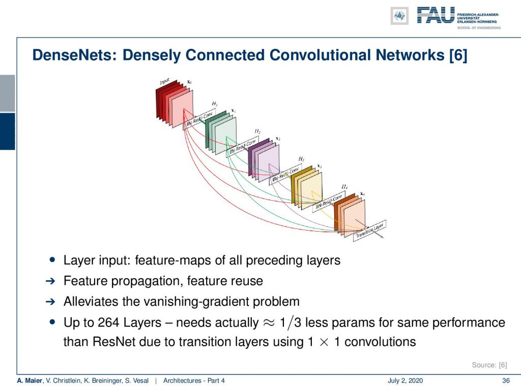
With DenseNets, you try to connect almost everything with everything. You have densely connected convolutional neural networks. It has feature propagation and feature reuse. It very much also alleviates the vanishing gradient problem and with up to 264 layers, you actually need one third fewer parameters for the same performance than ResNet due to the transition layers using 1×1 convolutions.
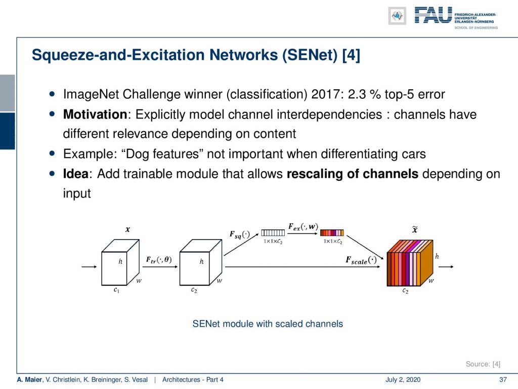
Also, a very interesting idea that I would like to show you are the squeeze and excitation networks, This is the ImageNet challenge winner in 2017 and it had 2.3% top-5-error. The idea is to explicitly model the channel interdependencies which means essentially that you have some channels that are more relevant depending on the content. If you have dog features, they will not be very interesting when you are trying to look at cars.
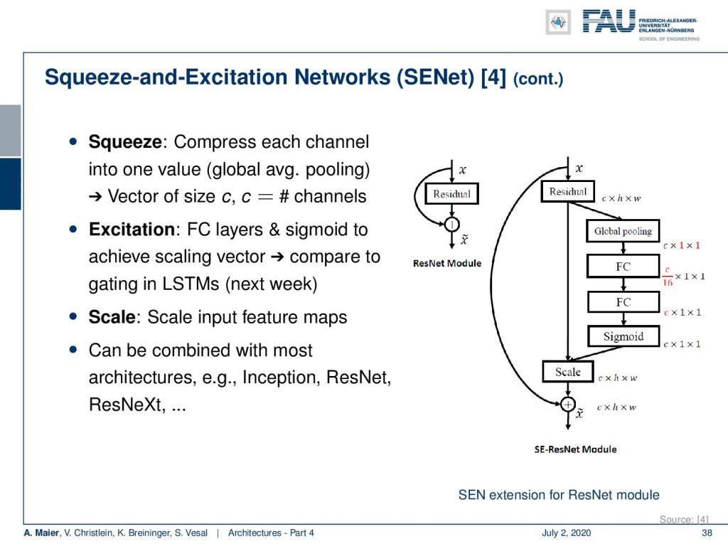
So, how is this implemented? Well, we add a trainable module that allows the rescaling of the channels depending on the input. So, we have the feature maps shown here. Then, we have the side branch that is mapping down only to a single dimension. The single dimension is then multiplied to the different feature maps allowing for some feature maps to be suppressed depending on the input and other feature maps to be scaled up depending on the input. We essentially squeeze, i.e., we compress each channel into one value by global average pooling. So this is how we construct the feature importance and then we excite where required. We use fully connected layers in the sigmoid function in order to excite only the important ones. By the way, this is very similar to what we would be doing in gating in the long short term memory cells which we’ll talk about probably in one of the videos next week. Then we scale so we scale the input maps with the output.

We can combine this of course with most other architectures: With inception modules, with ResNet, with ResNeXt, etc. So, plenty of different options that we could go for. To be honest, I don’t want to show you another architecture here.
What we’ll do next time is we talk about learning network architectures. So, there are ways to determine this automatically. Wouldn’t that be much more efficient? Well, stay tuned I will tell you in the next video!
If you liked this post, you can find more essays here, more educational material on Machine Learning here, or have a look at our Deep LearningLecture. I would also appreciate a follow on YouTube, Twitter, Facebook, or LinkedIn in case you want to be informed about more essays, videos, and research in the future. This article is released under the Creative Commons 4.0 Attribution License and can be reprinted and modified if referenced.
References
[1] Klaus Greff, Rupesh K. Srivastava, and Jürgen Schmidhuber. “Highway and Residual Networks learn Unrolled Iterative Estimation”. In: International Conference on Learning Representations (ICLR). Toulon, Apr. 2017. arXiv: 1612.07771.
[2] Kaiming He, Xiangyu Zhang, Shaoqing Ren, et al. “Deep Residual Learning for Image Recognition”. In: 2016 IEEE Conference on Computer Vision and Pattern Recognition (CVPR). Las Vegas, June 2016, pp. 770–778. arXiv: 1512.03385.
[3] Kaiming He, Xiangyu Zhang, Shaoqing Ren, et al. “Identity mappings in deep residual networks”. In: Computer Vision – ECCV 2016: 14th European Conference, Amsterdam, The Netherlands, 2016, pp. 630–645. arXiv: 1603.05027.
[4] J. Hu, L. Shen, and G. Sun. “Squeeze-and-Excitation Networks”. In: ArXiv e-prints (Sept. 2017). arXiv: 1709.01507 [cs.CV].
[5] Gao Huang, Yu Sun, Zhuang Liu, et al. “Deep Networks with Stochastic Depth”. In: Computer Vision – ECCV 2016, Proceedings, Part IV. Cham: Springer International Publishing, 2016, pp. 646–661.
[6] Gao Huang, Zhuang Liu, and Kilian Q. Weinberger. “Densely Connected Convolutional Networks”. In: 2017 IEEE Conference on Computer Vision and Pattern Recognition (CVPR). Honolulu, July 2017. arXiv: 1608.06993.
[7] Alex Krizhevsky, Ilya Sutskever, and Geoffrey E Hinton. “ImageNet Classification with Deep Convolutional Neural Networks”. In: Advances In Neural Information Processing Systems 25. Curran Associates, Inc., 2012, pp. 1097–1105. arXiv: 1102.0183.
[8] Yann A LeCun, Léon Bottou, Genevieve B Orr, et al. “Efficient BackProp”. In: Neural Networks: Tricks of the Trade: Second Edition. Vol. 75. Berlin, Heidelberg: Springer Berlin Heidelberg, 2012, pp. 9–48.
[9] Y LeCun, L Bottou, Y Bengio, et al. “Gradient-based Learning Applied to Document Recognition”. In: Proceedings of the IEEE 86.11 (Nov. 1998), pp. 2278–2324. arXiv: 1102.0183.
[10] Min Lin, Qiang Chen, and Shuicheng Yan. “Network in network”. In: International Conference on Learning Representations. Banff, Canada, Apr. 2014. arXiv: 1102.0183.
[11] Olga Russakovsky, Jia Deng, Hao Su, et al. “ImageNet Large Scale Visual Recognition Challenge”. In: International Journal of Computer Vision 115.3 (Dec. 2015), pp. 211–252.
[12] Karen Simonyan and Andrew Zisserman. “Very Deep Convolutional Networks for Large-Scale Image Recognition”. In: International Conference on Learning Representations (ICLR). San Diego, May 2015. arXiv: 1409.1556.
[13] Rupesh Kumar Srivastava, Klaus Greff, Urgen Schmidhuber, et al. “Training Very Deep Networks”. In: Advances in Neural Information Processing Systems 28. Curran Associates, Inc., 2015, pp. 2377–2385. arXiv: 1507.06228.
[14] C. Szegedy, Wei Liu, Yangqing Jia, et al. “Going deeper with convolutions”. In: 2015 IEEE Conference on Computer Vision and Pattern Recognition (CVPR). June 2015, pp. 1–9.
[15] C. Szegedy, V. Vanhoucke, S. Ioffe, et al. “Rethinking the Inception Architecture for Computer Vision”. In: 2016 IEEE Conference on Computer Vision and Pattern Recognition (CVPR). June 2016, pp. 2818–2826.
[16] Christian Szegedy, Sergey Ioffe, and Vincent Vanhoucke. “Inception-v4, Inception-ResNet and the Impact of Residual Connections on Learning”. In: Thirty-First AAAI Conference on Artificial Intelligence (AAAI-17) Inception-v4, San Francisco, Feb. 2017. arXiv: 1602.07261.
[17] Andreas Veit, Michael J Wilber, and Serge Belongie. “Residual Networks Behave Like Ensembles of Relatively Shallow Networks”. In: Advances in Neural Information Processing Systems 29. Curran Associates, Inc., 2016, pp. 550–558. A.
[18] Di Xie, Jiang Xiong, and Shiliang Pu. “All You Need is Beyond a Good Init: Exploring Better Solution for Training Extremely Deep Convolutional Neural Networks with Orthonormality and Modulation”. In: 2017 IEEE Conference on Computer Vision and Pattern Recognition (CVPR). Honolulu, July 2017. arXiv: 1703.01827.
[19] Lingxi Xie and Alan Yuille. Genetic CNN. Tech. rep. 2017. arXiv: 1703.01513.
[20] Sergey Zagoruyko and Nikos Komodakis. “Wide Residual Networks”. In: Proceedings of the British Machine Vision Conference (BMVC). BMVA Press, Sept. 2016, pp. 87.1–87.12.
[21] K Zhang, M Sun, X Han, et al. “Residual Networks of Residual Networks: Multilevel Residual Networks”. In: IEEE Transactions on Circuits and Systems for Video Technology PP.99 (2017), p. 1.
[22] Barret Zoph, Vijay Vasudevan, Jonathon Shlens, et al. Learning Transferable Architectures for Scalable