
Residual Networks
These are the lecture notes for FAU’s YouTube Lecture “Deep Learning“. This is a full transcript of the lecture video & matching slides. We hope, you enjoy this as much as the videos. Of course, this transcript was created with deep learning techniques largely automatically and only minor manual modifications were performed. If you spot mistakes, please let us know!
Welcome back to deep learning! Today we want to discuss a little more architectures and in particular the really deep ones. So, we are really going towards deep learning. If you want to train deeper models with all the things that we’ve seen so far, you see that we go into a certain kind of saturation. If you want to go deeper, then you just add layers on top and you would hope that the training error would go down. But if you look very carefully, you can see that a 20 layer network has a lower training error and also a lower test set error than for example a 56 layer model. So we cannot just increase the layers and layers and layers and hope that things get better. This effect is not just caused by overfitting. We are building layers on top. So, there must be other reasons and it’s likely that these reasons are related to the vanishing gradient problem. Other reasons could be the ReLU, the initialization, or the problem of the internal covariate shift where we tried batch normalization, ELU, and SELU, but we still have a problem with the poor propagation of activations and gradients. We see that if you try to build those very deep models, we get problems with vanishing gradients and we can’t train early layers which even results in a worse loss on the training set.
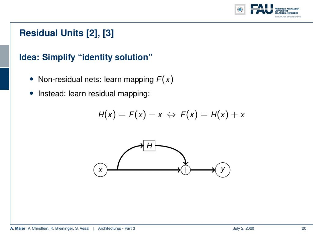
So, I have one solution for you and these are residual units. They are a very cool idea. So, what they propose to do is not learn the direct mapping F(x), but instead, we learn the residual mapping. So, we want to learn H(x) and H(x) is the difference between F(x) and x. So, we can also express it in a different way and this is actually how it’s implemented. You compute your network F(x) as some layer H(x) + x. So, the trainable part is now essentially in a side branch and the side branch is H(x) that’s the trainable one. On the main branch, we have just some x plus the side branch that will deliver our estimated y.
In the original implementation of residual blocks, there was still a difference. It was not exactly like we had it on the previous slide. So we had the side branch where we have a weighting layer, batch normalization, ReLU, weighting, another batch normalization, followed by the addition and another non-linearity, the ReLU for one residual block. This was later then changed into using batch norm, ReLU, weight, batch norm, ReLU, and weight for the residual block. It turned out that this kind of configuration was more stable. We essentially have the identity that is backpropagated on the plus branch. So, this is very nice because we can then propagate the gradient back into the early layers just because of this addition and we get a much more stable backpropagation this way.
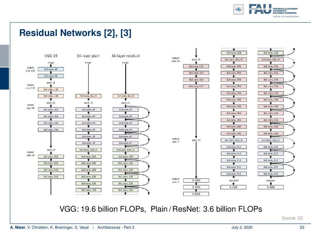
This then brings us to a complete residual network. So, we cut it at the bottom and show the bottom part on the right-hand side. This is a comparison between VGG, the 43 layers plain network, and the 43 layers residual network. You can see that there are essentially these skip connections that are being introduced. They allow us to skip over this step and then backpropagate in the respective earlier layers. There’s also downsampling involved and then, of course, the skip connections also have to be downsampled. So, this is why we have dotted connections at these positions. We can see that VGG has some 19.6 billion FLOPs while our plain and residual networks have only 3.6 billion FLOPs. So, it’s also more efficient.
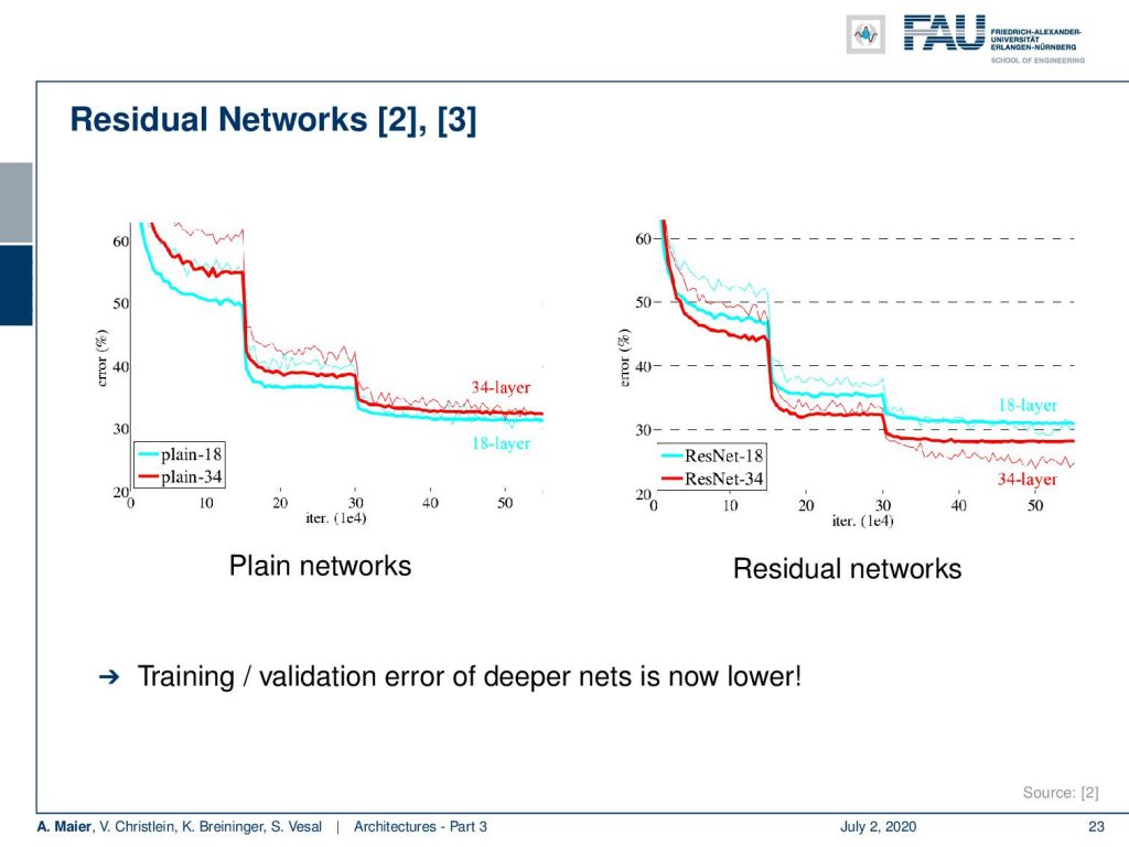
Now let’s put this to the test. We can now see that already in the 34 layers case, we don’t get the error rate as we would like to have them with very deep networks. So, the error is higher than if we only use an 18 layers network. But if you introduce the residual connections, we can see that we get a benefit and a reduced error rate. So, the residual connections help us to get more stable gradients and we can now get the training and the validation error lower with going deeper.
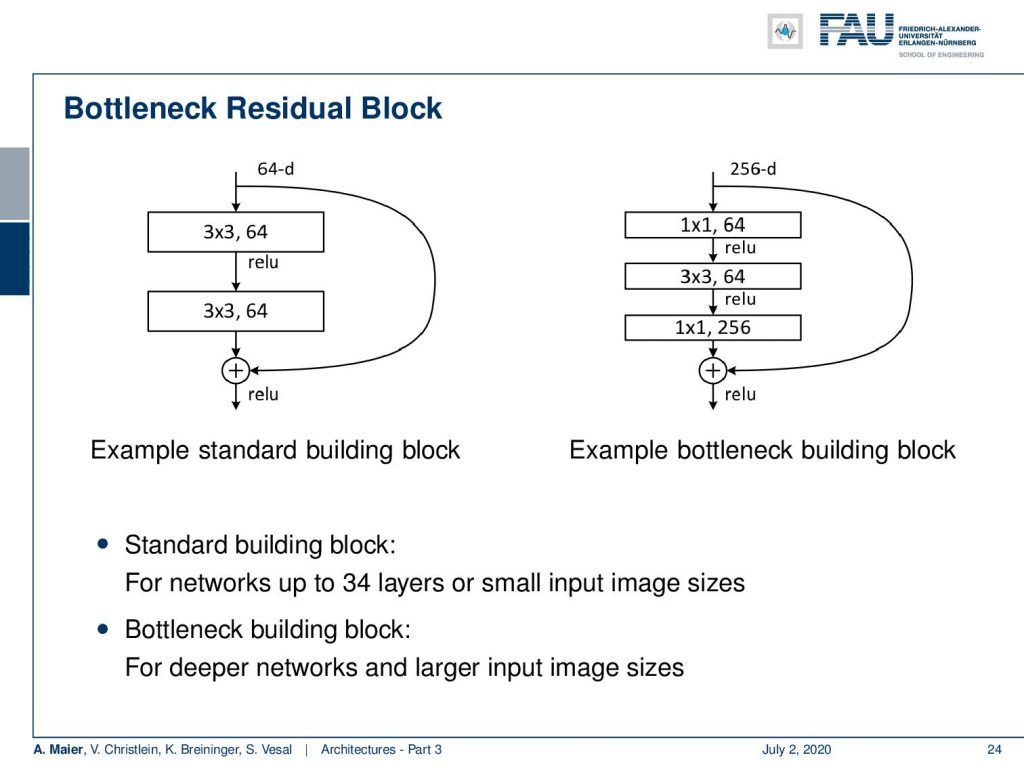
There are different variants of the residual block networks. There is the standard building block and here on the right-hand side, you can see that we can also use the bottleneck idea by downsampling channels, then doing the convolutions, and upsampling again. This is the kind of bottleneck version of the residual block.
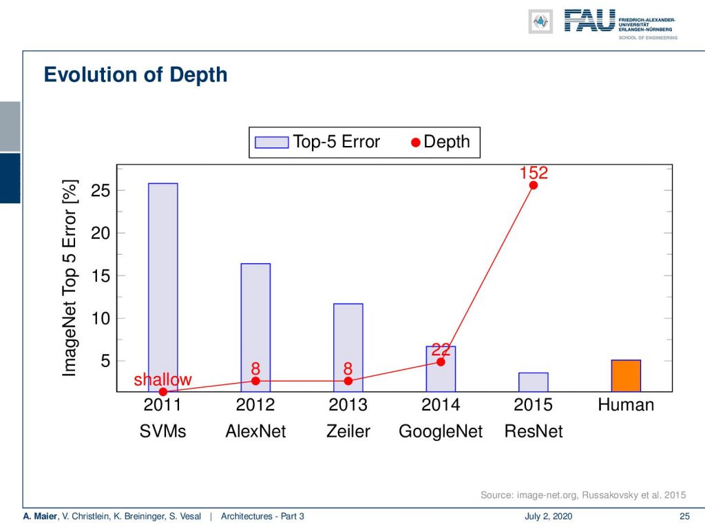
So, we can combine this with the other recipes that we have learned so far. If we do that, we can see that we can even train networks with a hundred and fifty-two layers. This then produced in 2015 one of the first networks that actually beat human performance. Remember all the things that we said about human performance, in particular, if you only have one label. So, actually you would have to have more labels to grasp the uncertainty of the problem. In any case, we can see here that we really go into the range of human performance and this is a very nice result.
People have been asking “Why do these residual networks perform so well?”. A very interesting interpretation is this so-called ensemble view of ResNets. So here, you can see that if we build residual layers or residual blocks on top of each other, we see that we can break this down into a kind of recursion. So, if we have x₃ equals x₂ plus H₃(x₂), we can resubstitute and see that this is equal to x₁ plus H₂(x₁) plus H₃(x₁ + H₂(x₁)). We can substitute again and see that we actually compute x₀ + H₁(x₀) plus H₂(x₀ + H₁(x₀)) plus H₃(x₀ + H₁(x₀) + H₂(x₀ + H₁(x₀))). Wow, very cool trick. This is something that you may want to remember if somebody is going to test you for whatever unknown reason about your knowledge of deep learning. So, I really would recommend having a close look at this line. So, we see in the interpretation that we are essentially constructing ensembles of our more shallow residual classifiers. So, we could say that our classifier trained from ResNets is essentially building a very strong ensemble.
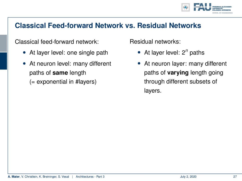
So this is very nice and we see that in a classical feed-forward network, we can change the representation in every single layer area because we have essentially this matrix multiplication in there. The matrix multiplication has the property that it can convert into a completely different domain. So, essentially in the classical feed-forward network, we have one single path and we have at neuron-level many different paths. In the residual networks, we get 2ⁿ paths. At neuron-level, we get many different paths of varying lengths going through different subsets of the layers which is a very strong ensemble that is constructed this way.
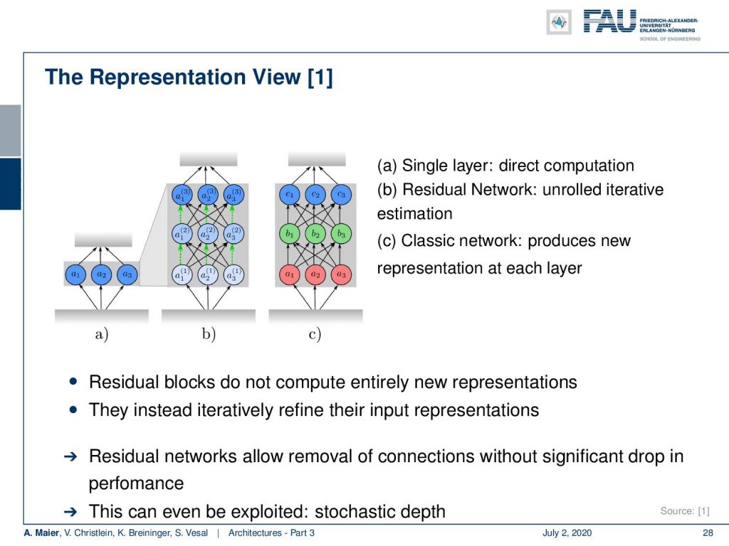
We can also change our viewpoint and think about the residual networks and the fully connected ones that we’ve seen earlier. In the fully connected layers, you can essentially change the complete representation. So we’re trying to show this here in a) b) and c). So a) would be just one conversion from one domain into another. If we now unroll this, we can see that the residual network is essentially doing a gradual change in representation over the different layers. So, we see that we have a slight change and then the color gradually changes towards blue where we have to decide for the representation in the very end. If we compare this to fully connected layers like in c), we can have a completely different representation in the first layer followed by a completely different representation in the second layer, and lastly, we finally map on to the desired representation in the last layer. So in the classical fully connected ones, we can produce a completely new representation in every layer. This means that they also become very dependent because the representation needs to be matching in order to do further processing.
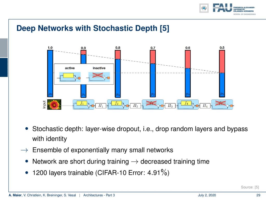
So, we can do a very interesting experiment like a lesion study as you would do in a biological neural network. Here are some results with stochastic depth. So, the idea is now that we turn off entire layers. We can turn off complete layers and it doesn’t destroy the classification that is done by the ResNet which is pretty cool. So, if you’ll just turn off like 10% of the layers, then you can see that we have a reduction in performance but it doesn’t break down. The more layers I’m reducing, the worse the performance gets, but because we have this slight change of representation, we can knock off individual steps and it doesn’t completely destroy this network. So, this is of course something that we would expect from an ensemble. Alright, with these humble representations and this gradual change we will later in this class show that ResNets can also be interpreted as a kind of gradient descent procedure. It is of course because related to the observation that if you follow a gradient descent, then we have the same gradual change from every position. As a result, we are constructing essentially something similar with the ResNet. We can actually show that the ResNet configuration can also be arrived at if you seek to optimize an unknown loss function. You want to train this gradient and you will exactly come up with a ResNet as a solution. But this will take a bit of time and we will talk about this towards the end of this class. So far, these networks have been built really really deep. There are even 1200 layers possible even on CIFAR-10. So that’s a very interesting result. We see that we are really going towards very deep networks.
So what else could we talk about? Well, next time in deep learning, we want to talk about the rise of residual connections and a couple of more tricks that help you build really effective deep networks. So, I hope you enjoyed this video and tune in for the next one!
If you liked this post, you can find more essays here, more educational material on Machine Learning here, or have a look at our Deep LearningLecture. I would also appreciate a follow on YouTube, Twitter, Facebook, or LinkedIn in case you want to be informed about more essays, videos, and research in the future. This article is released under the Creative Commons 4.0 Attribution License and can be reprinted and modified if referenced.
References
[1] Klaus Greff, Rupesh K. Srivastava, and Jürgen Schmidhuber. “Highway and Residual Networks learn Unrolled Iterative Estimation”. In: International Conference on Learning Representations (ICLR). Toulon, Apr. 2017. arXiv: 1612.07771.
[2] Kaiming He, Xiangyu Zhang, Shaoqing Ren, et al. “Deep Residual Learning for Image Recognition”. In: 2016 IEEE Conference on Computer Vision and Pattern Recognition (CVPR). Las Vegas, June 2016, pp. 770–778. arXiv: 1512.03385.
[3] Kaiming He, Xiangyu Zhang, Shaoqing Ren, et al. “Identity mappings in deep residual networks”. In: Computer Vision – ECCV 2016: 14th European Conference, Amsterdam, The Netherlands, 2016, pp. 630–645. arXiv: 1603.05027.
[4] J. Hu, L. Shen, and G. Sun. “Squeeze-and-Excitation Networks”. In: ArXiv e-prints (Sept. 2017). arXiv: 1709.01507 [cs.CV].
[5] Gao Huang, Yu Sun, Zhuang Liu, et al. “Deep Networks with Stochastic Depth”. In: Computer Vision – ECCV 2016, Proceedings, Part IV. Cham: Springer International Publishing, 2016, pp. 646–661.
[6] Gao Huang, Zhuang Liu, and Kilian Q. Weinberger. “Densely Connected Convolutional Networks”. In: 2017 IEEE Conference on Computer Vision and Pattern Recognition (CVPR). Honolulu, July 2017. arXiv: 1608.06993.
[7] Alex Krizhevsky, Ilya Sutskever, and Geoffrey E Hinton. “ImageNet Classification with Deep Convolutional Neural Networks”. In: Advances In Neural Information Processing Systems 25. Curran Associates, Inc., 2012, pp. 1097–1105. arXiv: 1102.0183.
[8] Yann A LeCun, Léon Bottou, Genevieve B Orr, et al. “Efficient BackProp”. In: Neural Networks: Tricks of the Trade: Second Edition. Vol. 75. Berlin, Heidelberg: Springer Berlin Heidelberg, 2012, pp. 9–48.
[9] Y LeCun, L Bottou, Y Bengio, et al. “Gradient-based Learning Applied to Document Recognition”. In: Proceedings of the IEEE 86.11 (Nov. 1998), pp. 2278–2324. arXiv: 1102.0183.
[10] Min Lin, Qiang Chen, and Shuicheng Yan. “Network in network”. In: International Conference on Learning Representations. Banff, Canada, Apr. 2014. arXiv: 1102.0183.
[11] Olga Russakovsky, Jia Deng, Hao Su, et al. “ImageNet Large Scale Visual Recognition Challenge”. In: International Journal of Computer Vision 115.3 (Dec. 2015), pp. 211–252.
[12] Karen Simonyan and Andrew Zisserman. “Very Deep Convolutional Networks for Large-Scale Image Recognition”. In: International Conference on Learning Representations (ICLR). San Diego, May 2015. arXiv: 1409.1556.
[13] Rupesh Kumar Srivastava, Klaus Greff, Urgen Schmidhuber, et al. “Training Very Deep Networks”. In: Advances in Neural Information Processing Systems 28. Curran Associates, Inc., 2015, pp. 2377–2385. arXiv: 1507.06228.
[14] C. Szegedy, Wei Liu, Yangqing Jia, et al. “Going deeper with convolutions”. In: 2015 IEEE Conference on Computer Vision and Pattern Recognition (CVPR). June 2015, pp. 1–9.
[15] C. Szegedy, V. Vanhoucke, S. Ioffe, et al. “Rethinking the Inception Architecture for Computer Vision”. In: 2016 IEEE Conference on Computer Vision and Pattern Recognition (CVPR). June 2016, pp. 2818–2826.
[16] Christian Szegedy, Sergey Ioffe, and Vincent Vanhoucke. “Inception-v4, Inception-ResNet and the Impact of Residual Connections on Learning”. In: Thirty-First AAAI Conference on Artificial Intelligence (AAAI-17) Inception-v4, San Francisco, Feb. 2017. arXiv: 1602.07261.
[17] Andreas Veit, Michael J Wilber, and Serge Belongie. “Residual Networks Behave Like Ensembles of Relatively Shallow Networks”. In: Advances in Neural Information Processing Systems 29. Curran Associates, Inc., 2016, pp. 550–558. A.
[18] Di Xie, Jiang Xiong, and Shiliang Pu. “All You Need is Beyond a Good Init: Exploring Better Solution for Training Extremely Deep Convolutional Neural Networks with Orthonormality and Modulation”. In: 2017 IEEE Conference on Computer Vision and Pattern Recognition (CVPR). Honolulu, July 2017. arXiv: 1703.01827.
[19] Lingxi Xie and Alan Yuille. Genetic CNN. Tech. rep. 2017. arXiv: 1703.01513.
[20] Sergey Zagoruyko and Nikos Komodakis. “Wide Residual Networks”. In: Proceedings of the British Machine Vision Conference (BMVC). BMVA Press, Sept. 2016, pp. 87.1–87.12.
[21] K Zhang, M Sun, X Han, et al. “Residual Networks of Residual Networks: Multilevel Residual Networks”. In: IEEE Transactions on Circuits and Systems for Video Technology PP.99 (2017), p. 1.
[22] Barret Zoph, Vijay Vasudevan, Jonathon Shlens, et al. Learning Transferable Architectures for Scalable