
Modern Activations
These are the lecture notes for FAU’s YouTube Lecture “Deep Learning“. This is a full transcript of the lecture video & matching slides. We hope, you enjoy this as much as the videos. Of course, this transcript was created with deep learning techniques largely automatically and only minor manual modifications were performed. If you spot mistakes, please let us know!
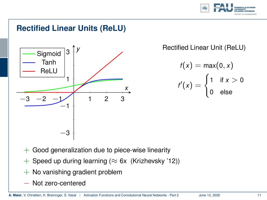
Welcome back to Part 2 of activation functions and convolutional neural networks! Now, we want to continue talking about the activation functions and the new ones used in deep learning. One of the most famous examples is the rectified linear unit (ReLU). Now the ReLU, we are already encountered earlier and the idea is simply to set the negative half-space to zero and the positive half-space to x. This then results in derivatives of one for the entire positive half-space and zero everywhere else. So, this is very nice because this way we get a good generalization. Due to the piecewise linearity, there’s a significant speedup. The function can be evaluated very quickly because we don’t need the exponential functions that are typically a bit slow on the implementation side. We don’t have this vanishing gradient problem because we have really large areas of high values for the derivative of this function. A drawback is it’s not zero centered. Now, this has not been solved with the rectified linear unit. However these ReLUs, they were a big step forward. With ReLUs, you could for the first time build deeper networks and with deeper networks, I mean networks that have more hidden layers than three.
Typically in classical machine learning, neural networks were limited to approximately three layers because already at this point you get the vanishing gradient problem. The lower layers never seen any of the gradients and therefore never updated their weights. So, ReLUs enabled the training of deep nets without unsupervised pre-training. You could already build deep nets, but you had to do unsupervised pre-training, With ReLUs, you could train from scratch directly just putting your data in which was a big step forward. Also, the implementation is very easy because the first derivative is 1 if the unit is activated and 0 otherwise. So there’s no second-order effect.
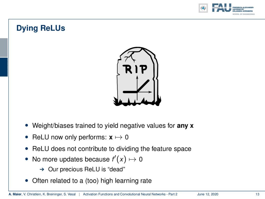
One problem still remains: Dying ReLUs. If you have weights and biases trained to yield negative results for x, then you simply always end up with a zero derivative. The ReLU always generates a zero output and this means that they no longer contribute to your training process. So, it simply stops at this point and no updates are possible because of the 0 derivative. This precious ReLU is suddenly always 0 and can no longer be trained. This is also quite frequently happening if you have a too high learning rate. Here, you may want to be careful with setting learning rates. There are a couple of ways out of this which we will discuss in the next couple of videos.
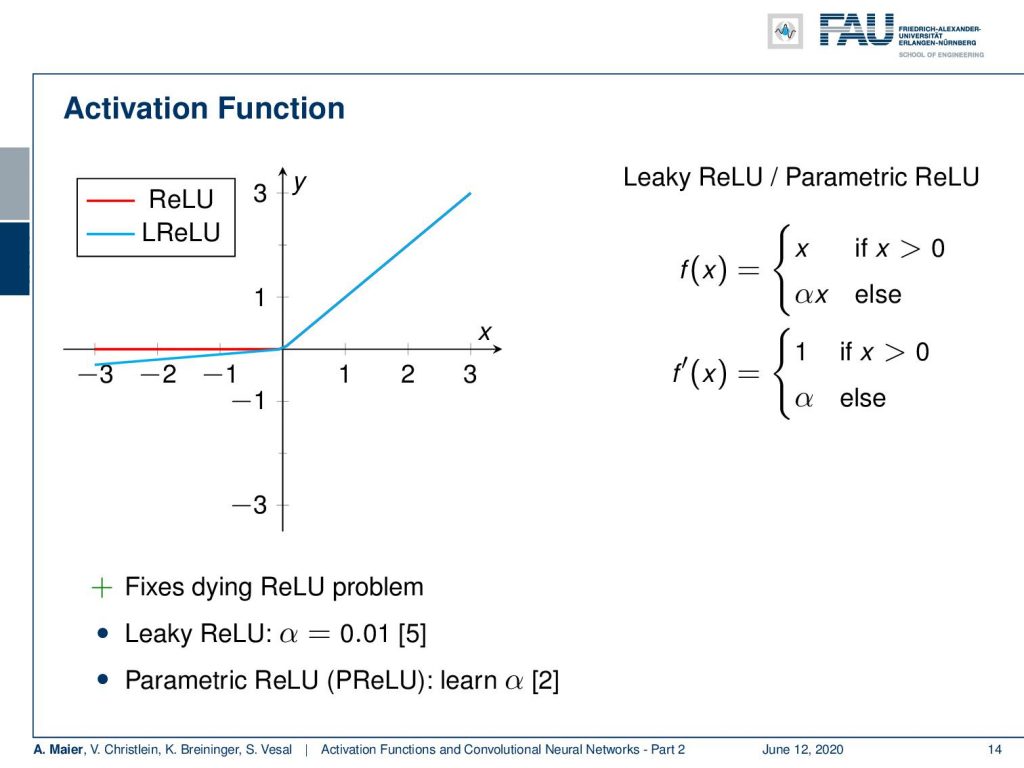
One way to alleviate the problem is already using not just a ReLU but something that is called leaky or parametric ReLU. The approach here is that you not set the negative half-space to zero but you set it to a scaled small number. So, you take α times x and you set α to be a small number. Then, you have a very similar effect as the ReLU, but you don’t end up with the dying ReLU problem as the derivative is never zero but it’s α. I first typically set the values to 0.01. The parametric ReLU is a further extension. Here, you make α a trainable parameter. So you can actually learn for every activation function how large it should be.
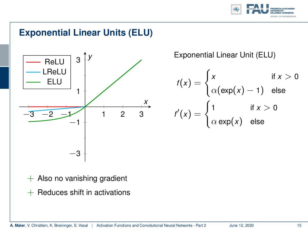
There are also exponential linear units and here the idea is that you find a smooth function on the negative half-space that slowly decays. You can see here, we set it to α times exponent of x minus one. This then results in derivatives 1 and α exponent x. So also, an interesting way to get a saturating effect. Here, we have no vanishing gradient and it also reduces the shift in activations because we can get also negative output values.
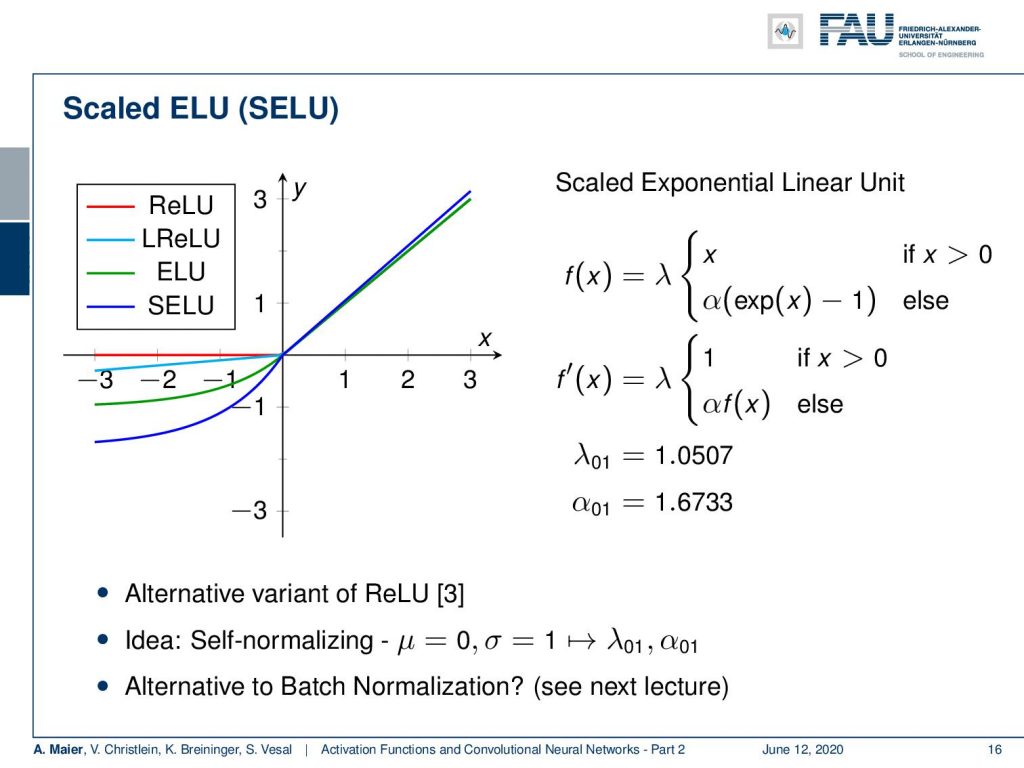
If you choose this variant of the exponential linear unit you add an additional scaling λ. If you have inputs with zero mean and unit variance, you can choose α and λ with these two values as reported here and they will preserve a zero mean and unit variance. So, this scaled exponential function (SELU) also gets rid of the problem of the internal covariate shift. So it’s an alternative variant of the ReLU and the nice property is that if you have these zero mean unit variance inputs, then your activations will remain on the same scale. You don’t have to care about the internal covariate shift. Another thing that we can do about the internal covariate shift is bach normalization. This is something that we’ll talk about in a couple of videos.
Okay, what other activation functions are there? There is maxout that learns the activation function. There are radial basis functions that can be employed. There is softplus which is a logarithm of 1 plus e to the power of x that was found to be less efficient than the ReLU.

This is actually getting ridiculous, isn’t it? So, what should we use now? People even went this far that they were trying to find the optimal activation function. They used reinforcement learning search in order to find them.
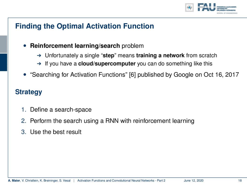
We will talk about reinforcement learning in a later lecture. We’ll just discuss the results here. One problem in this reinforcement learning type of setup is that it’s computationally very expensive. In every step of the reinforcement training procedure, you have to train an entire network from scratch. So, you need a supercomputer to do something like this, and searching for activation functions is reference [6]. It was published by Google already in 2017 and they actually did this. So, the strategy was to define the search space then perform the search using a recurrent neural network with reinforcement learning and in the end, they want to use the best result.
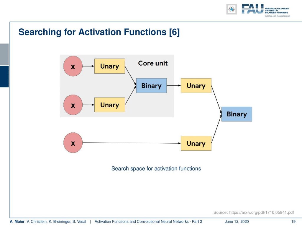
The search space that they used is that they put in x into some unary functions. Then these unary functions were combined using a binary core unit. This could then be merged again unary with another instance of x that was then used to produce to the final output using a binary function. So, this is essentially the search space that they went through. Of course, they took this kind of modeling because you can explain a lot of the typical activation functions like the sigmoid and so on using these kinds of expressions.
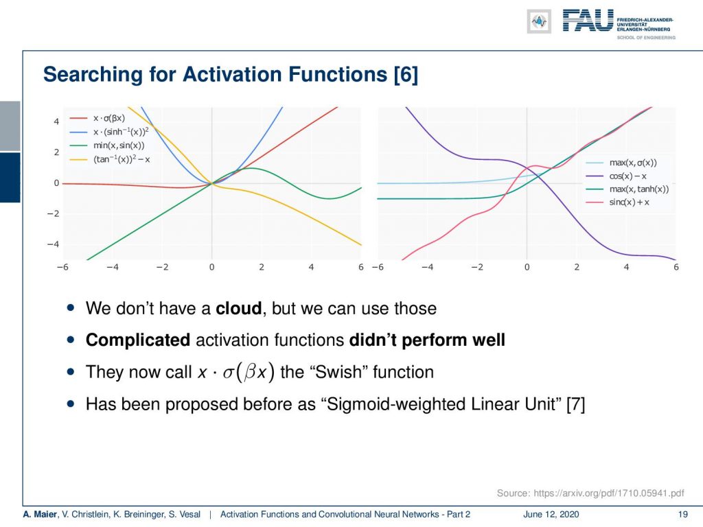
We see that these are activation functions that they found useful. So, we can’t do the procedure ourselves, but we can of course look at the results that they found. Here are some examples and interestingly you can see that some of the results that they produced resulted even no longer in convex functions. One general result that he came up with is that complicated activation functions generally didn’t perform very well. They found something that is x times σ(β x) which they call the swish function. So, this seemed to be performing quite well and actually this function that they identified using the search has already been proposed before as the sigmoid weighted linear unit [7].
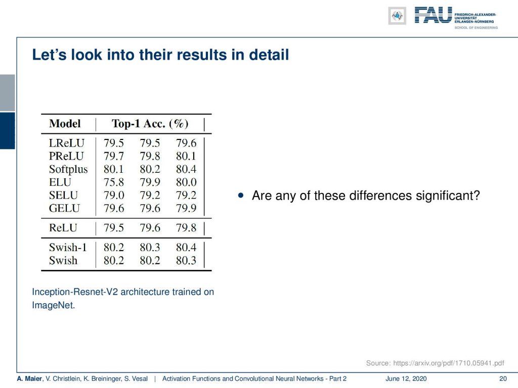
So let’s look into the results in detail. Now a disclaimer: Never show tables in your results. Try hard to find a better representation! However, we did not find a better representation. What I can show you here is these are the top one accuracies that they have obtained. This was done in an inception Resnet v2 architecture trained on ImageNet. In the third row from the bottom, you could see the results with the ReLU and then the bottom two rows show the results with swish-1 and swish. Now, the question that we want to ask is: “Are these changes actually significant?” So, significance means that you compute the probability of the observation to be a result of randomness and you want to make sure that the result that you’re reporting is not random. In this entire chain of processing, we have frequently random initializations, ee have a lot of steps that may have introduced sampling errors, and so on. So you really want to make sure that the result is not random. Therefore, we have significance tests. If you look very closely, you really ask yourself: “Are the changes that are reported here actually significant?”.
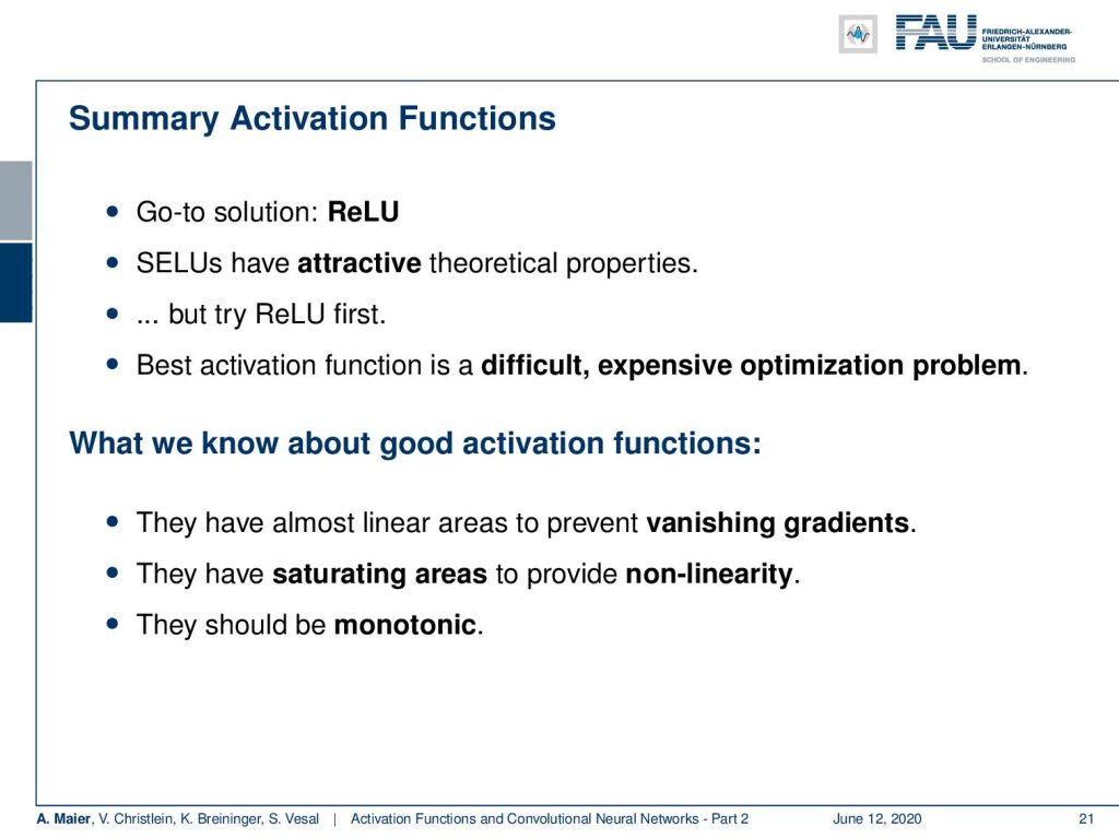
Therefore our recommendation is to go to the ReLU. They work really well and if you have some problems, you can choose to use batch normalization which we’ll talk about in one of the next videos. Another interesting thing is the scaled exponential linear unit because it has this self-adaptation property. So, this is really attractive but try ReLU first. This is really typically the way you want to go. The search for the best activation function is a difficult and extensive optimization problem which has not led us to much better activation functions. So what we already have here is sufficient for most of your problems. What we do know about good activation functions is what we know from these observations: They have almost linear areas to prevent vanishing gradients, they have saturating areas to provide non-linearity, and they should be monotonic as this is really useful for our optimization.
This already brings us to the preview on the next lecture. In the next lecture, we really want to go towards convolutional neural networks and see into the tricks how we can reduce the number of connections and also the number of parameters for building really deep networks. So, I hope you liked this lecture and I am looking forward to seeing you in the next one!
If you liked this post, you can find more essays here, more educational material on Machine Learning here, or have a look at our Deep Learning Lecture. I would also appreciate a clap or a follow on YouTube, Twitter, Facebook, or LinkedIn in case you want to be informed about more essays, videos, and research in the future. This article is released under the Creative Commons 4.0 Attribution License and can be reprinted and modified if referenced.
References
[1] I. J. Goodfellow, D. Warde-Farley, M. Mirza, et al. “Maxout Networks”. In: ArXiv e-prints (Feb. 2013). arXiv: 1302.4389 [stat.ML].
[2] Kaiming He, Xiangyu Zhang, Shaoqing Ren, et al. “Delving Deep into Rectifiers: Surpassing Human-Level Performance on ImageNet Classification”. In: CoRR abs/1502.01852 (2015). arXiv: 1502.01852.
[3] Günter Klambauer, Thomas Unterthiner, Andreas Mayr, et al. “Self-Normalizing Neural Networks”. In: Advances in Neural Information Processing Systems (NIPS). Vol. abs/1706.02515. 2017. arXiv: 1706.02515.
[4] Min Lin, Qiang Chen, and Shuicheng Yan. “Network In Network”. In: CoRR abs/1312.4400 (2013). arXiv: 1312.4400.
[5] Andrew L. Maas, Awni Y. Hannun, and Andrew Y. Ng. “Rectifier Nonlinearities Improve Neural Network Acoustic Models”. In: Proc. ICML. Vol. 30. 1. 2013.
[6] Prajit Ramachandran, Barret Zoph, and Quoc V. Le. “Searching for Activation Functions”. In: CoRR abs/1710.05941 (2017). arXiv: 1710.05941.
[7] Stefan Elfwing, Eiji Uchibe, and Kenji Doya. “Sigmoid-weighted linear units for neural network function approximation in reinforcement learning”. In: arXiv preprint arXiv:1702.03118 (2017).
[8] Christian Szegedy, Wei Liu, Yangqing Jia, et al. “Going Deeper with Convolutions”. In: CoRR abs/1409.4842 (2014). arXiv: 1409.4842.