
Confounders & Adversarial Attacks
These are the lecture notes for FAU’s YouTube Lecture “Deep Learning“. This is a full transcript of the lecture video & matching slides. We hope, you enjoy this as much as the videos. Of course, this transcript was created with deep learning techniques largely automatically and only minor manual modifications were performed. Try it yourself! If you spot mistakes, please let us know!
So welcome back to deep learning! Today, I want to talk about more visualization techniques. But actually, I want to start motivating why we need visualization techniques in the next couple of minutes.
Okay, here we go. Visualization and Attention Mechanisms – Part 2. Visualization of parameters and the first thing is the motivation. So, the network’s learn a representation of the training data but the question is of course what happens with the data in our network.
This is really an important thing and you should really care about this because it’s very useful to investigate unintentional and unexpected behavior. One thing that I really want to highlight here is adversarial examples. Of course, you want to figure out why your network performs really well in the lab but it fails in the wild. So, this is also an important thing that you want to be solving. Then, you can figure out potential causes for this because if you look into these visualization techniques, they will help you to identify focus on wrong types of features, noise properties, and things like that. So, we’ll have a couple of examples in the next videos. I want to show you some anecdotal examples.

For example the identification of tanks in photos. so this is actually an example from Neil Fraser’s website, a Google developer. I’m not entirely sure if this really happened or whether this is just an urban legend. So the legend goes like this: People and the Pentagon wanted to train a neural network to identify tanks on images. What could you do in order to construct such a net? Well, you go out there and then you take images of tanks and then you take images of non-tank situations. Well, typically you would expect them to be in some scenery. So, you go out into the forest and take some pictures. Then, of course, you have to get some pictures of tanks. Tanks you typically find on on a battlefield and there’s you know smoke around, mud, dirty and gritty. So, you collect your images of tanks and then you have maybe 200 of the forest images and 200 of the tank images. You’ll go back to your lab and then you train your deep neural network or maybe not so deep if you only have this very small data set. You go ahead and you get an almost perfect classification rate. So, everybody’s very happy it seems that your system is working really well,
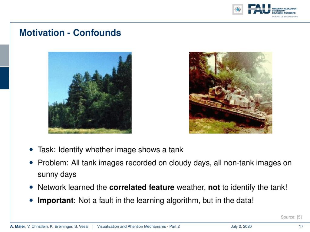
So, I have two examples here on this slide and you were saying “Yeah! I’ve solved the problem!” So, let’s build a real system from this and this will warn us of tanks. They built the system and they realized it didn’t work at all in practice. They actually had a recognition rate of approximately 50 percent in this two-class problem. This means this is approximately random guessing. So, what could have possibly gone wrong? Well, if you look at those images you can see that all of the forest images have essentially all been taken on sunny nice weather days. Then, of course, you see that the tanks have been taken on days that are more cloudy. You know there are not so good weather conditions. Of course, when you see tanks, they fire, there are grenades around, and, of course, this means that there will be smoke and other things happening.
So, what the system essentially learned is not to identify tanks, but it took the shortcut. Here, the shortcut is that you try to detect the weather. So, if you have a blue sky, good weather conditions, very few noise in the image, then it’s potentially a non-tank image. If you have noise and bad lighting conditions, then it’s potentially a tank image. Obviously, this kind of classification system doesn’t help at all for the task of detecting tanks. So, we can summarize this the network simply learned the data has a correlated feature. This is typically called a confounding factor. It did not identify the tank. So, the important lesson here is: This is not a fault in the learning algorithm but in the data. So, also when you go out and collect your data you should be extremely careful that you have representative data of the future application.
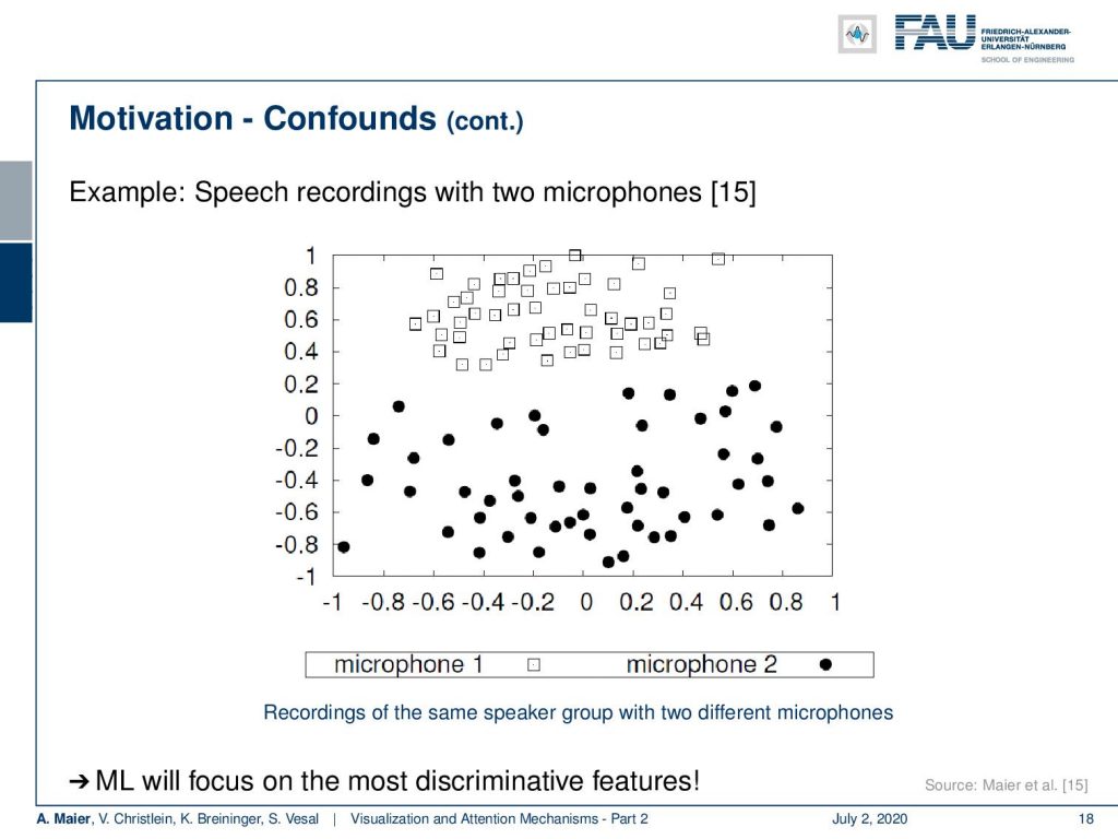
I have another example here for confounders. What you see here in this visualization are speech recordings. This is a dimensional scaling. So, what we try to do here is to map different speakers into a 2-D space. We map an entire recording onto a single point. What you should actually see here are 51 dots one for each speaker. You see that we have black dots and we have squares. Now, the squares have been recorded with Microphone 1 and the dots have been recorded with Microphone 2. These are exactly the same speakers and even worse: These are even simultaneously recorded instances but with two different microphones. One microphone was very close to the mouth of the speakers and the other microphone was located on a video camera approximately two and a half meters away from the speaker. Here you can see that the microphone characteristic is a clear confounder and you can very easily separate the two groups of speakers although they are exactly the same speakers by the microphone.
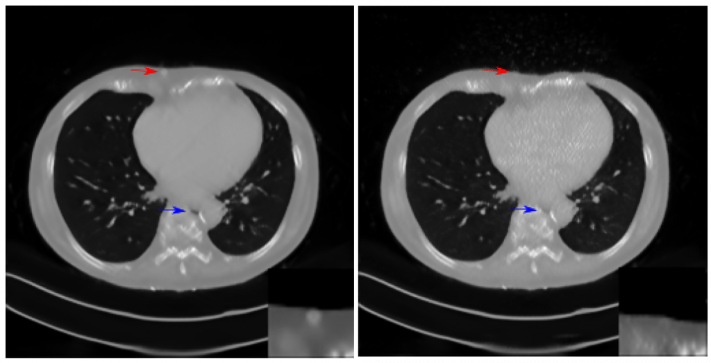
Now, imagine you do something similar for detecting pathology. You collect all of the speakers with the pathology with one microphone and all of the speakers without the pathology with another microphone. Then it’s likely that your system will learn to identify the different microphones instead of the pathology. Of course, this is not only the case with microphones. Think of using two different scanners for creating medical images like scanning histopathology. You have different types of pathology and you scan each type with a different scanner. Maybe they are just located in two different hospitals because the patients with Disease A go to Hospital A and the patients of Disease B go to Hospital B. Then, you have a massive confounder in here because all of the patients with Disease A have been scanned by Scanner A and all the controls or Disease B patients have been scanned by Scanner B. So, it’s again likely that you will learn to differentiate the scanner for example by identifying a characteristic noise pattern instead of identifying the disease.

The same is true for cameras. You can even show that in image forensics if you have images taken with the same digital camera, then only by the specific noise pattern in the pixels, you can identify that specific camera. These are of course local things that are very easily picked up by a deep neural network. In particular, in the early layers so be very careful if you collect data. You need to collect from multiple different sites make sure that you have representative data. Imagine you train a classifier for COVID-19 and all of the scans with the COVID-19 patients came out of a specific region and all the positive samples are taken with let’s say a set of 3-4 scanners. Then you compare this to non-COVID-19 patients and if they are acquired on a different scanner or even different sites, you might very, very easily introduce a recognition of these scanners instead of a recognition of the disease.
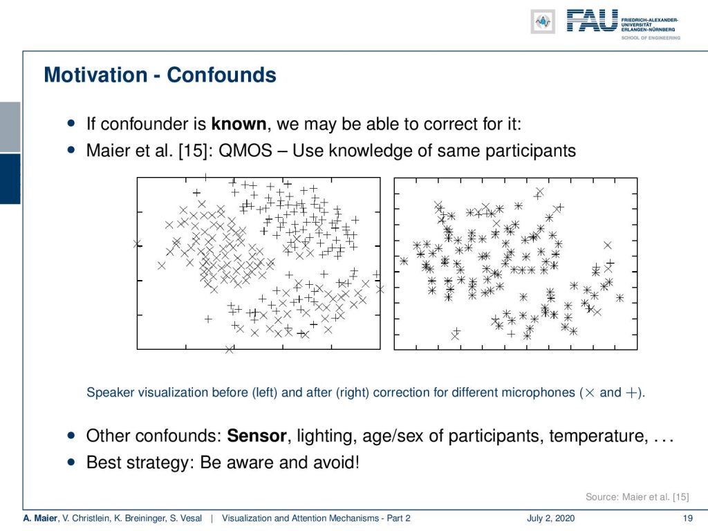
So be very careful, look at the data, and try to understand if there’s the risk for confounders. Of course, try to omit them. We have proposed a technique actually to counter confounders and this is what we have in [15]. Here, the idea is that you actively include the information about the confounder and try to suppress it, here, for the visualization. Then, you can show that you can actually remove the bias that is introduced by microphones for example. So, you have to be aware of the confounders which might be sensors, lighting conditions, age, the gender of participants, temperature – yes even temperature is likely to produce an influence on the sensory machinery.
So be careful. All of these conditions can be confounded and if you have confounders in the data you have to compensate for them or you try to avoid them in your data collection. So, please be aware of these problems these are very likely to spoil your entire classification system. If you don’t look at the data carefully, you will never figure out where the problem is.
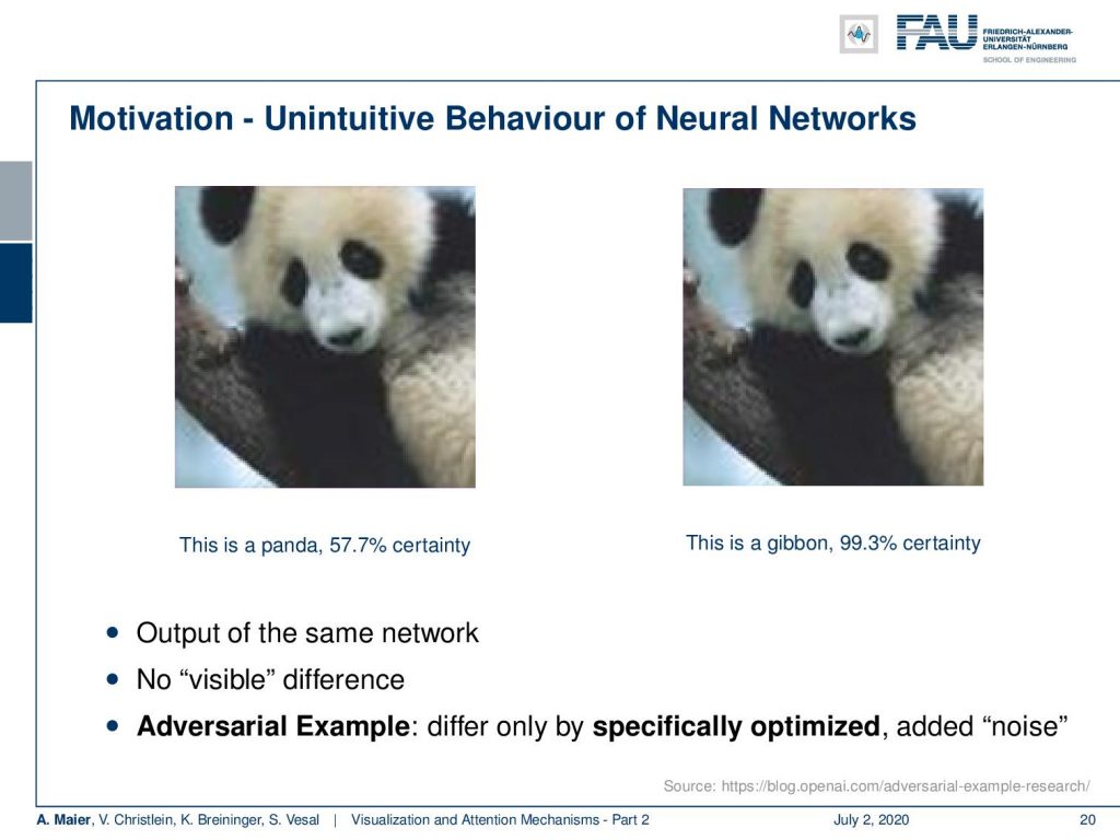
Another big problem that you encounter in machine learning and deep learning systems is the problems with adversarial examples. Then, you have unintuitive behavior. We show you two images here. For the left image, our neural network believes at the confidence of 57% that this is a panda. On the right image which looks almost the same to us, it is at 99.3% certain that this is a Gibbon. Now, how can this be true? These two inputs look almost the same.
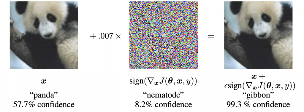
What happens with the right image is that somebody was attacking the neural network. They introduced a noise pattern onto the image which is only one or two gray values in each color channel but the noise pattern was constructed with knowledge about the deep neural network. What they did is they essentially tried to increase the output for the class given maximally by introducing random-like inputs. What you can actually do is if you know the entire network, you can design this additional noise pattern in a way that will maximize the excitation for the wrong class. For humans, this is absolutely not recognizable.
The way it works is that it accumulates over the different layers of the small inputs at every pixel but averaged and added up over the different layers. It allows us to introduce a small shift and then the small shift over the layers can increase to actually force the network to go to the wrong decision. So, you could argue that this adversarial example is a kind of flaw in the network. We want to prevent, of course, such adversary examples. Well, actually we will see that this is not possible because they are created by optimization. You will always end up with adversarial examples.
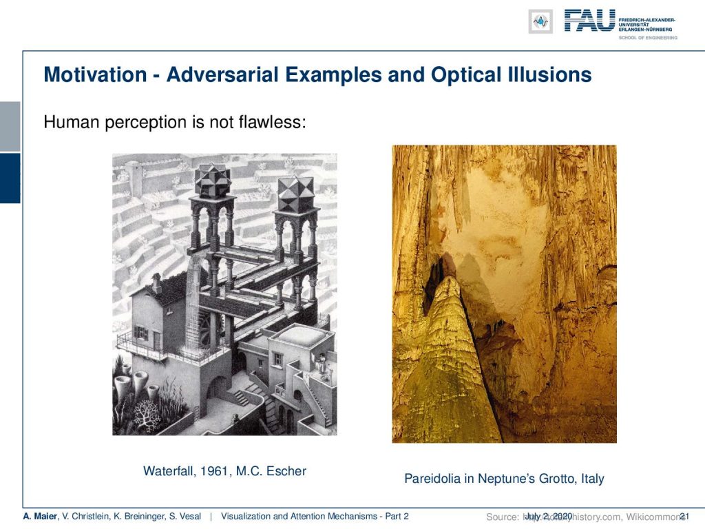
So, why does this happen? Well, we could argue that adversarial examples are somehow like optical illusions. So also, human perception is not flawless. Here on the left-hand side, you see this waterfall by Escher. If you follow the structure, you will see that the waterfall is feeding this structure itself and it’s essentially an infinite loop. Here, the optical illusion is that if we look at the individual parts, we will find them consistent, but of course, the entire image is not consistent. Still, we look at the part and find them plausible. A slightly better example of an adversarial example is maybe the image here on the right. This is actually Neptune’s grotto in Italy. People call this shadow that is created by these stone formations the “organ player”. If you look closely at the shadow, it looks like there is a person sitting and playing the stone formation as an organ player would do. So, optical illusions also exist in human beings and adversarial examples are essentially the equivalent in deep neural networks.
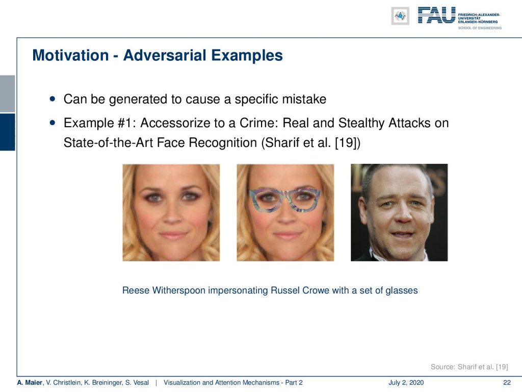
In contrast to the optical illusions, we can construct those adversarial examples. So, I already hinted at this. They are generated to cause a specific mistake and here is another example. This is an attack on state-of-the-art face recognition which you find in [19]. What they did is they defined a set of pixels which essentially takes the shape of glasses. These glasses now can be adjusted. So, they can assign arbitrary color values and they choose the color values in a way that would lead to the wrong identification. You can show if an image of Reese Witherspoon, you add these magical glasses, and you can see that they are really colorful. So, they create large inputs and they specifically strengthen activations that then lead to a wrong classification. With these particular glasses, you can see that Reese Witherspoon now successfully disguised as Russell Crowe. You may say “Wow, this is complete nonsense and this can’t be! I can still see Reese Witherspoon!” Well, yes. You can still see Reese Witherspoon because the human perceptual system works differently than this neural network that is trained for person identification. There are even works that build on top of this. They actually printed these fancy glasses and they also showed that camera-based person identification systems can be tricked for such strange attacks.

There’s even more to that. This is the so-called “toaster sticker”. The toaster sticker is used to misguide generally networks trained on ImageNet. So, it has been designed in order to lead to a classification towards the class “toaster”. Now, if you print this toaster sticker, here, you can see, this is a fancy colorful image. You just put it into the scene and the toaster sticker will cause classification of the class “toaster”. It does not only work on one specific architecture. They could actually show that it works over several kinds of architectures. This toaster sticker could not only fool a single network but several networks that have all been trained on ImageNet. So, in the top image, you see the network works correctly. It classifies a banana. You add the toaster sticker and it classifies toaster. Interestingly, the paper even has an attachment where you can download the toaster sticker and print it yourself and try it on your own ImageNet networks.
Ok, so this is essentially the summary of the motivation. We see that sometimes there are strange things happening in deep neural networks. We would like to understand why they occur and what the problem is. This can be done through visualization techniques. You want to identify confounders, you want to explain why our network works, or why it doesn’t, and you want to increase the confidence in predictions.
So next time, we will actually look into different visualization techniques. We’ll start with the more simple ones which are then followed by optimization-based and gradient-based techniques. We will only look into activation based techniques in the next video. So, thank you very much for listening and see you in the next video. Bye-bye!
If you liked this post, you can find more essays here, more educational material on Machine Learning here, or have a look at our Deep LearningLecture. I would also appreciate a follow on YouTube, Twitter, Facebook, or LinkedIn in case you want to be informed about more essays, videos, and research in the future. This article is released under the Creative Commons 4.0 Attribution License and can be reprinted and modified if referenced. If you are interested in generating transcripts from video lectures try AutoBlog.

Links
Yosinski et al.: Deep Visualization Toolbox
Olah et al.: Feature Visualization
Adam Harley: MNIST Demo
References
[1] Dzmitry Bahdanau, Kyunghyun Cho, and Yoshua Bengio. “Neural Machine Translation by Jointly Learning to Align and Translate”. In: 3rd International Conference on Learning Representations, ICLR 2015, San Diego, 2015.
[2] T. B. Brown, D. Mané, A. Roy, et al. “Adversarial Patch”. In: ArXiv e-prints (Dec. 2017). arXiv: 1712.09665 [cs.CV].
[3] Jianpeng Cheng, Li Dong, and Mirella Lapata. “Long Short-Term Memory-Networks for Machine Reading”. In: CoRR abs/1601.06733 (2016). arXiv: 1601.06733.
[4] Jacob Devlin, Ming-Wei Chang, Kenton Lee, et al. “BERT: Pre-training of Deep Bidirectional Transformers for Language Understanding”. In: CoRR abs/1810.04805 (2018). arXiv: 1810.04805.
[5] Neil Frazer. Neural Network Follies. 1998. URL: https://neil.fraser.name/writing/tank/ (visited on 01/07/2018).
[6] Ross B. Girshick, Jeff Donahue, Trevor Darrell, et al. “Rich feature hierarchies for accurate object detection and semantic segmentation”. In: CoRR abs/1311.2524 (2013). arXiv: 1311.2524.
[7] Alex Graves, Greg Wayne, and Ivo Danihelka. “Neural Turing Machines”. In: CoRR abs/1410.5401 (2014). arXiv: 1410.5401.
[8] Karol Gregor, Ivo Danihelka, Alex Graves, et al. “DRAW: A Recurrent Neural Network For Image Generation”. In: Proceedings of the 32nd International Conference on Machine Learning. Vol. 37. Proceedings of Machine Learning Research. Lille, France: PMLR, July 2015, pp. 1462–1471.
[9] Nal Kalchbrenner, Lasse Espeholt, Karen Simonyan, et al. “Neural Machine Translation in Linear Time”. In: CoRR abs/1610.10099 (2016). arXiv: 1610.10099.
[10] L. N. Kanal and N. C. Randall. “Recognition System Design by Statistical Analysis”. In: Proceedings of the 1964 19th ACM National Conference. ACM ’64. New York, NY, USA: ACM, 1964, pp. 42.501–42.5020.
[11] Andrej Karpathy. t-SNE visualization of CNN codes. URL: http://cs.stanford.edu/people/karpathy/cnnembed/ (visited on 01/07/2018).
[12] Alex Krizhevsky, Ilya Sutskever, and Geoffrey E Hinton. “ImageNet Classification with Deep Convolutional Neural Networks”. In: Advances In Neural Information Processing Systems 25. Curran Associates, Inc., 2012, pp. 1097–1105. arXiv: 1102.0183.
[13] Thang Luong, Hieu Pham, and Christopher D. Manning. “Effective Approaches to Attention-based Neural Machine Translation”. In: Proceedings of the 2015 Conference on Empirical Methods in Natural Language Lisbon, Portugal: Association for Computational Linguistics, Sept. 2015, pp. 1412–1421.
[14] A. Mahendran and A. Vedaldi. “Understanding deep image representations by inverting them”. In: 2015 IEEE Conference on Computer Vision and Pattern Recognition (CVPR). June 2015, pp. 5188–5196.
[15] Andreas Maier, Stefan Wenhardt, Tino Haderlein, et al. “A Microphone-independent Visualization Technique for Speech Disorders”. In: Proceedings of the 10th Annual Conference of the International Speech Communication Brighton, England, 2009, pp. 951–954.
[16] Volodymyr Mnih, Nicolas Heess, Alex Graves, et al. “Recurrent Models of Visual Attention”. In: CoRR abs/1406.6247 (2014). arXiv: 1406.6247.
[17] Chris Olah, Alexander Mordvintsev, and Ludwig Schubert. “Feature Visualization”. In: Distill (2017). https://distill.pub/2017/feature-visualization.
[18] Prajit Ramachandran, Niki Parmar, Ashish Vaswani, et al. “Stand-Alone Self-Attention in Vision Models”. In: arXiv e-prints, arXiv:1906.05909 (June 2019), arXiv:1906.05909. arXiv: 1906.05909 [cs.CV].
[19] Mahmood Sharif, Sruti Bhagavatula, Lujo Bauer, et al. “Accessorize to a Crime: Real and Stealthy Attacks on State-of-the-Art Face Recognition”. In: Proceedings of the 2016 ACM SIGSAC Conference on Computer and Communications CCS ’16. Vienna, Austria: ACM, 2016, pp. 1528–1540. A.
[20] K. Simonyan, A. Vedaldi, and A. Zisserman. “Deep Inside Convolutional Networks: Visualising Image Classification Models and Saliency Maps”. In: International Conference on Learning Representations (ICLR) (workshop track). 2014.
[21] J.T. Springenberg, A. Dosovitskiy, T. Brox, et al. “Striving for Simplicity: The All Convolutional Net”. In: International Conference on Learning Representations (ICRL) (workshop track). 2015.
[22] Dmitry Ulyanov, Andrea Vedaldi, and Victor S. Lempitsky. “Deep Image Prior”. In: CoRR abs/1711.10925 (2017). arXiv: 1711.10925.
[23] Ashish Vaswani, Noam Shazeer, Niki Parmar, et al. “Attention Is All You Need”. In: CoRR abs/1706.03762 (2017). arXiv: 1706.03762.
[24] Kelvin Xu, Jimmy Ba, Ryan Kiros, et al. “Show, Attend and Tell: Neural Image Caption Generation with Visual Attention”. In: CoRR abs/1502.03044 (2015). arXiv: 1502.03044.
[25] Jason Yosinski, Jeff Clune, Anh Mai Nguyen, et al. “Understanding Neural Networks Through Deep Visualization”. In: CoRR abs/1506.06579 (2015). arXiv: 1506.06579.
[26] Matthew D. Zeiler and Rob Fergus. “Visualizing and Understanding Convolutional Networks”. In: Computer Vision – ECCV 2014: 13th European Conference, Zurich, Switzerland, Cham: Springer International Publishing, 2014, pp. 818–833.
[27] Han Zhang, Ian Goodfellow, Dimitris Metaxas, et al. “Self-Attention Generative Adversarial Networks”. In: Proceedings of the 36th International Conference on Machine Learning. Vol. 97. Proceedings of Machine Learning Research. Long Beach, California, USA: PMLR, Sept. 2019, pp. 7354–7363. A.