Gated Recurrent Units
These are the lecture notes for FAU’s YouTube Lecture “Deep Learning“. This is a full transcript of the lecture video & matching slides. We hope, you enjoy this as much as the videos. Of course, this transcript was created with deep learning techniques largely automatically and only minor manual modifications were performed. If you spot mistakes, please let us know!
Welcome back to deep learning! Today we want to talk a bit about gated recurrent units (GRUs), a simplification of the LSTM cell.

So again a neural network: Gated recurrent units. So the idea here is that the LSTM is, of course, great, but it has a lot of parameters and it’s kind of difficult to train.
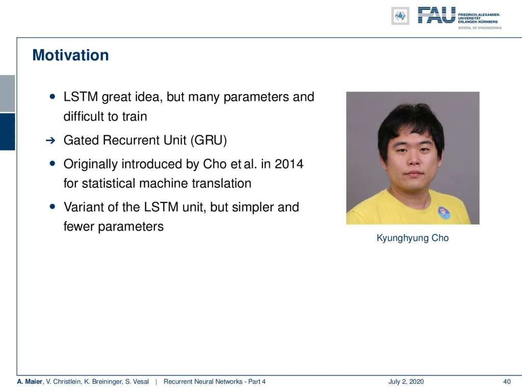
So, Cho came up with the gated recurrent unit and it was introduced in 2014 for statistical machine translation. You could argue it’s a kind of LSTM, but it’s simpler and it has fewer parameters.
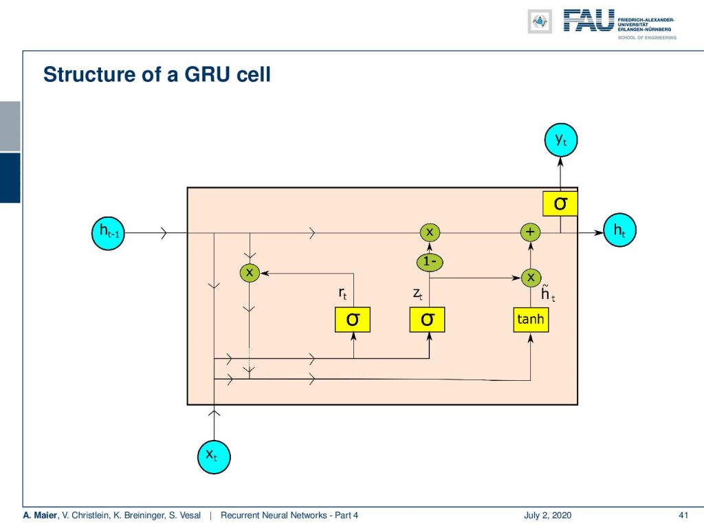
So this is the general setup. You can see we don’t have two different memories like in the LSTM. We only have one hidden state. One similarity to the LSTM is the hidden state flows only along a linear process. So, you only see multiplications and additions here. Again, as in the LSTM, we produce from the hidden state the output.
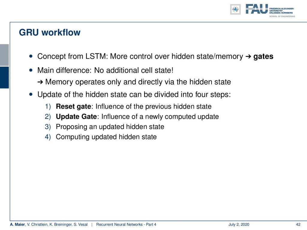
So let’s have a look into the ideas that Cho had in order to propose this cool cell. Well, it takes the concepts from the LSTM and it controls the memory by gates. The main difference is that there is no additional cell state. So, the memory only operates directly on the hidden state. The update of the state can be divided into four steps: There’s a reset gate that is controlling the influence of the previous hidden state. Then there is an update gate that introduces newly computed updates. So, the next step proposes an updated hidden state which is then used to update the hidden state.
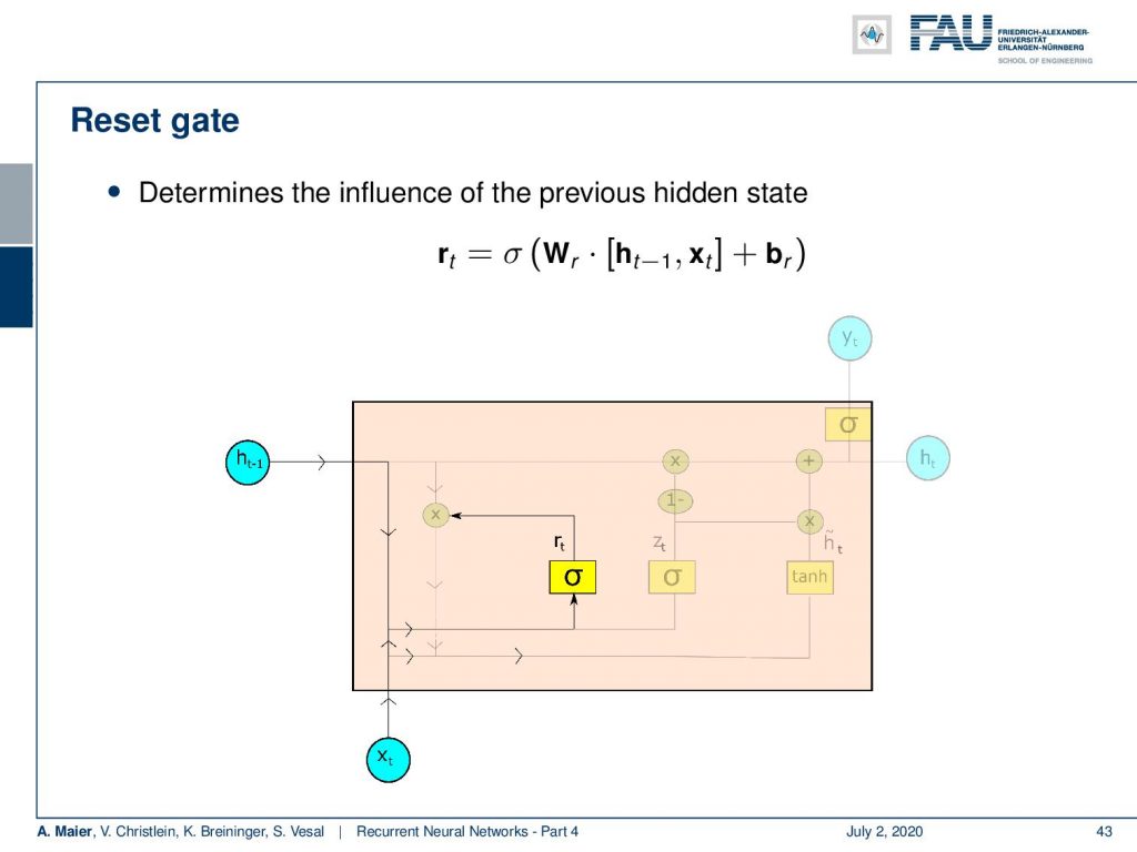
So, how does this work? Well, first we determine the influence of the previous hidden state. This is done by a sigmoid activation function. We again have a matrix-type of update. We concatenate the input and the previous hidden state multiplied with a matrix and add some bias. Then, feed it to this sigmoid activation function which produces some reset value r subscript t.
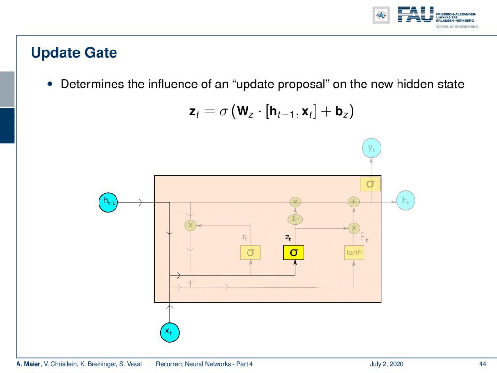
Next, we produce some z. This is essentially the update proposal on the new hidden state. So, this is again produced by a sigmoid function where we concatenate the last hidden state, and the input vector multiplied with a matrix W subscript z and add some bias.
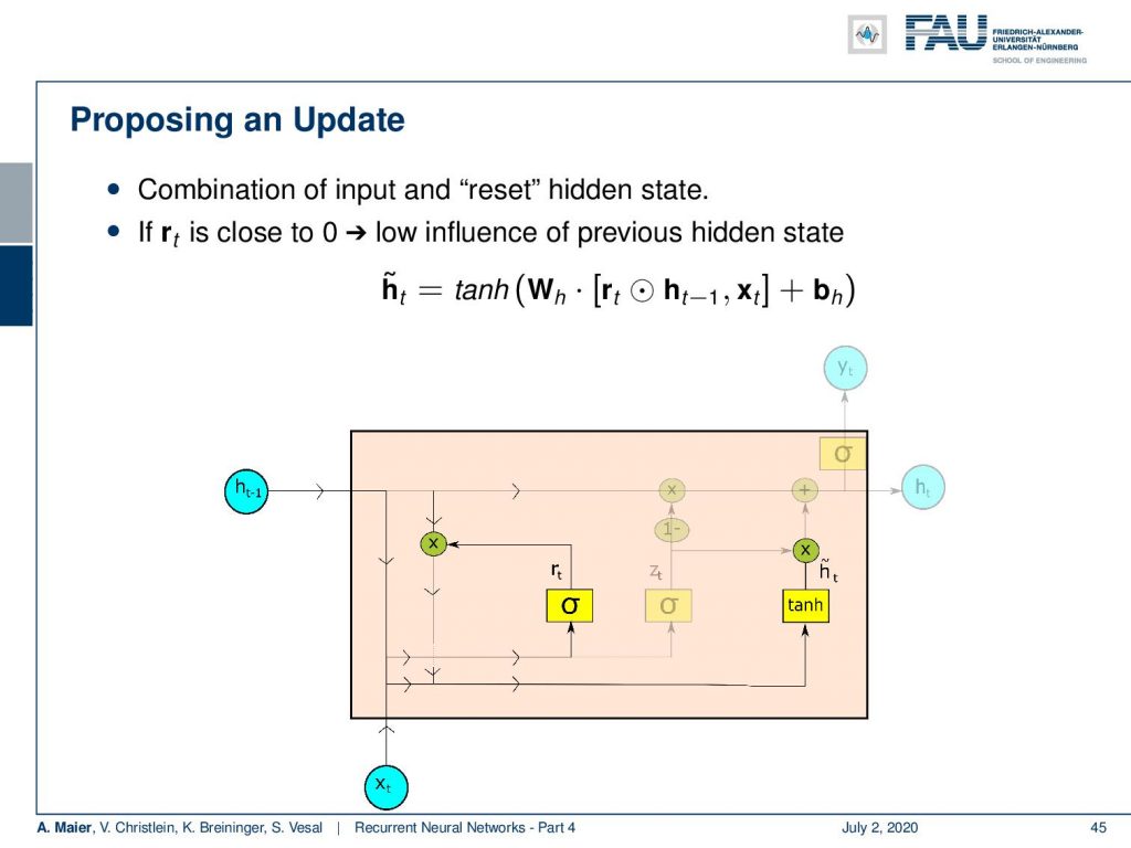
Next, we propose the update. So we combine the input and the reset state. This is done in the following manner: So, the update proposal h tilde is produced by a hyperbolic tangent where we take the reset gate times the last hidden state. So, we essentially remove entries that we don’t want to see from the last hidden state and concatenate x subscript t multiplied with some matrix W subscript h and add some bias b subscript h. This is then fed to a tanh to produce the update proposal.
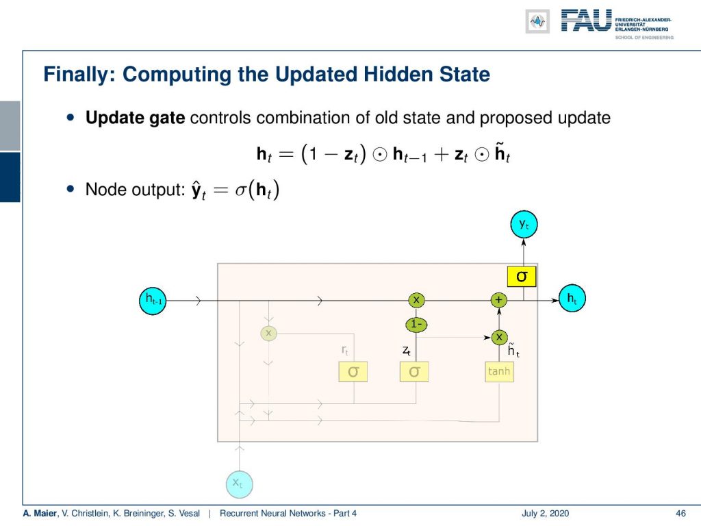
Now, with the update proposal, we go to the update gate. The update gate controls the combination of the old state and the proposed state. So, we compute the new state by multiplying 1 – z subscript t. You remember this is the intermediate variable that we computed earlier with the old state. Further, we add z subscript t times h tilde. This is the proposed update. So, essentially the sigmoid function that produced a z subscript t is now used to select whether to keep the old information from the old state or to update it with information from the new state. This gives the new hidden state. With the new hidden state, we produce the new output and notice again that we are omitting the transformation matrices in this step. So, we write this as sigmoid of h subscript t, but there’s actually the transformation matrices and biases. Noth we are not noting down here. So, this thing gives the final output y hat subscript t.
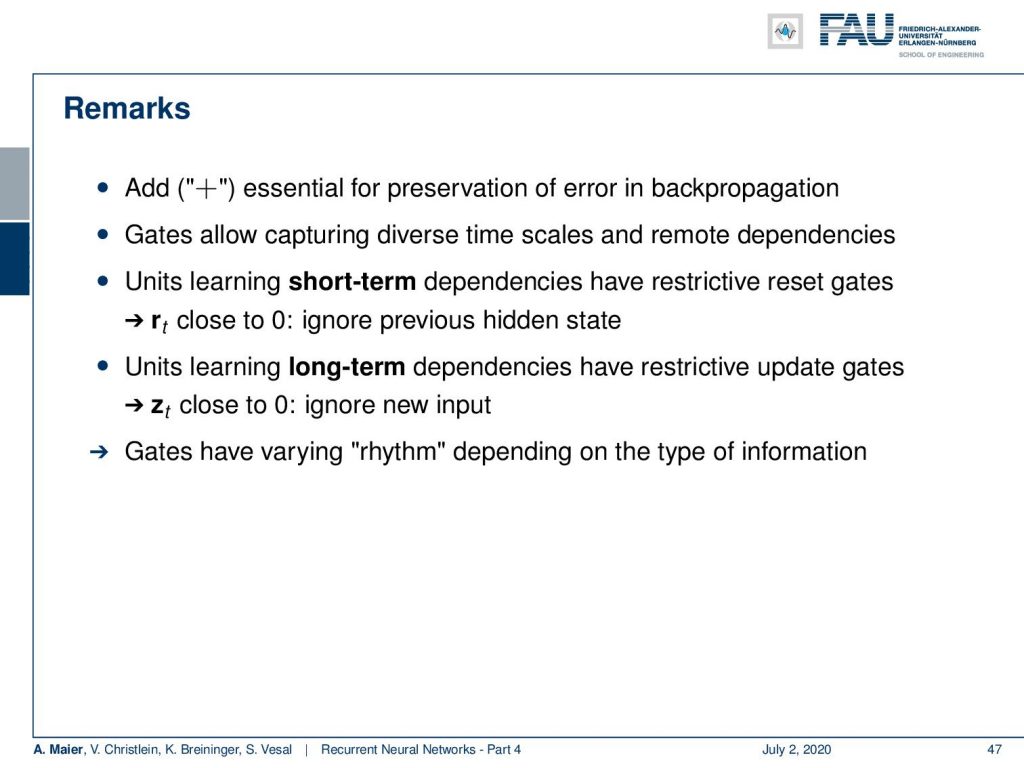
Some remarks: The addition is essential for the preservation of the error in the backpropagation. The gates allow capturing diverse timescales and remote dependencies. The units are able to learn short-term dependencies by learning restrictive gates. So, if we have an r subscript t close to zero it will ignore the previous hidden state. We can also learn long-term dependencies by having restrictive update gates. So, here we have the z subscript t close to zero which means we ignore new input the gates. Then, a varying rhythm depending on the type of information emerges. Now, you’d say “Ok. now we have our RNN units, we have LSTM units, and GRUs. So, which one should we take?”
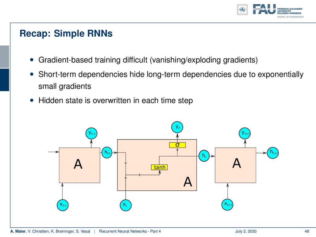
So, let’s have a short recap. In the simple RNNs, we had gradient-based training which was difficult to do. We had exploding gradients and vanishing gradient problems with long-term dependencies. Short-term dependencies were quite good but they could potentially hide the long-term dependencies due to exponentially small gradients and that the hidden state is overwritten in each time step.
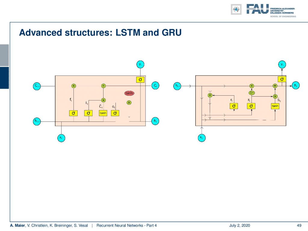
Then, we had LSTMs and GRUs. Both of them introduced gates that operate on memory. In LSTMs, we were splitting this into cell state and hidden state. In the GRU, we only have a hidden state. Both of them have memories that are completely linear which helps us with the long-term dependencies.
So, the similarities here, of course, are that the information is controlled by gates and the ability to capture dependencies of different time scales. The additive calculation of the state preserves the error during backpropagation. So, we can do more efficient training.
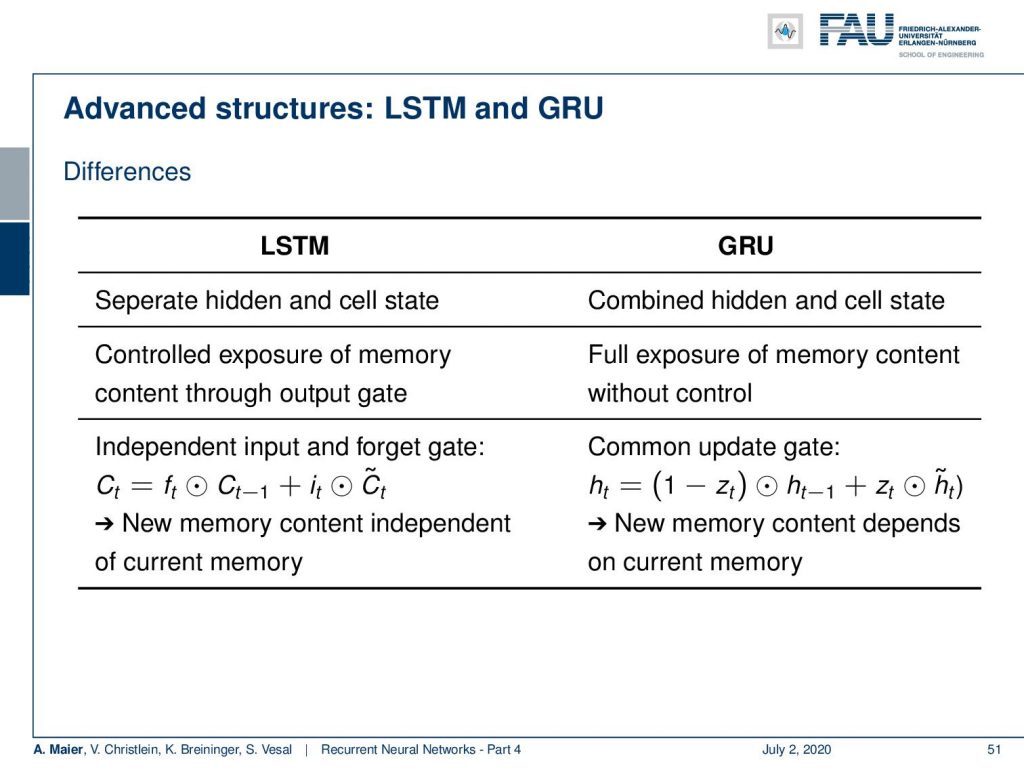
Of course, there are also differences the LSTMs have separate hidden and cell states. So, they control the exposure of the memory content through an output gate, an input, and a forget gate. They work independently. So, they could potentially do different things. New memory content is independent of the current memory. In the GRU, we have combined hidden and cell states. So, we have full exposure to the memory content without control. There is one common update gate that produces the new hidden state with our variable z subscript t. It essentially decides to either use the old state or to use the proposed update. So, the new memory content depends on the current memory.
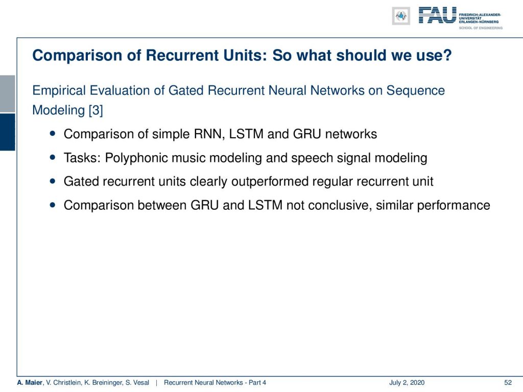
You can also compare the applications because you may ask so what should be used. In [3], you see an empirical evaluation of gated recurrent neural networks on sequence modeling. They compare the simple RNN, LSTMs, and GRU networks. The tasks were polyphonic music modeling and speech signal modeling. Results indicate that the gated recurrent units clearly outperformed the regular recurrent unit. The comparison between the GRU and the LSTM was not conclusive. They had a similar performance.
So, you could argue both of them are very well-suited for sequence modeling. One has fewer parameters but for the task presented in this paper, it didn’t make a big difference so both of them are viable options.
Well, next time in deep learning, we want to talk a bit about generating sequences. We now have recurrent neural networks and the recurrency can, of course, not be used just to process long sequences, but, of course, we can also generate sequences. Thus, we will look a bit into sequence generation. So thank you very much for listening. I hope you like this video and hope to see you in the next one. Bye-bye!
If you liked this post, you can find more essays here, more educational material on Machine Learning here, or have a look at our Deep LearningLecture. I would also appreciate a follow on YouTube, Twitter, Facebook, or LinkedIn in case you want to be informed about more essays, videos, and research in the future. This article is released under the Creative Commons 4.0 Attribution License and can be reprinted and modified if referenced.
RNN Folk Music
FolkRNN.org
MachineFolkSession.com
The Glass Herry Comment 14128
Links
Character RNNs
CNNs for Machine Translation
Composing Music with RNNs
References
[1] Dzmitry Bahdanau, Kyunghyun Cho, and Yoshua Bengio. “Neural Machine Translation by Jointly Learning to Align and Translate”. In: CoRR abs/1409.0473 (2014). arXiv: 1409.0473.
[2] Yoshua Bengio, Patrice Simard, and Paolo Frasconi. “Learning long-term dependencies with gradient descent is difficult”. In: IEEE transactions on neural networks 5.2 (1994), pp. 157–166.
[3] Junyoung Chung, Caglar Gulcehre, KyungHyun Cho, et al. “Empirical evaluation of gated recurrent neural networks on sequence modeling”. In: arXiv preprint arXiv:1412.3555 (2014).
[4] Douglas Eck and Jürgen Schmidhuber. “Learning the Long-Term Structure of the Blues”. In: Artificial Neural Networks — ICANN 2002. Berlin, Heidelberg: Springer Berlin Heidelberg, 2002, pp. 284–289.
[5] Jeffrey L Elman. “Finding structure in time”. In: Cognitive science 14.2 (1990), pp. 179–211.
[6] Jonas Gehring, Michael Auli, David Grangier, et al. “Convolutional Sequence to Sequence Learning”. In: CoRR abs/1705.03122 (2017). arXiv: 1705.03122.
[7] Alex Graves, Greg Wayne, and Ivo Danihelka. “Neural Turing Machines”. In: CoRR abs/1410.5401 (2014). arXiv: 1410.5401.
[8] Karol Gregor, Ivo Danihelka, Alex Graves, et al. “DRAW: A Recurrent Neural Network For Image Generation”. In: Proceedings of the 32nd International Conference on Machine Learning. Vol. 37. Proceedings of Machine Learning Research. Lille, France: PMLR, July 2015, pp. 1462–1471.
[9] Kyunghyun Cho, Bart Van Merriënboer, Caglar Gulcehre, et al. “Learning phrase representations using RNN encoder-decoder for statistical machine translation”. In: arXiv preprint arXiv:1406.1078 (2014).
[10] J J Hopfield. “Neural networks and physical systems with emergent collective computational abilities”. In: Proceedings of the National Academy of Sciences 79.8 (1982), pp. 2554–2558. eprint: http://www.pnas.org/content/79/8/2554.full.pdf.
[11] W.A. Little. “The existence of persistent states in the brain”. In: Mathematical Biosciences 19.1 (1974), pp. 101–120.
[12] Sepp Hochreiter and Jürgen Schmidhuber. “Long short-term memory”. In: Neural computation 9.8 (1997), pp. 1735–1780.
[13] Volodymyr Mnih, Nicolas Heess, Alex Graves, et al. “Recurrent Models of Visual Attention”. In: CoRR abs/1406.6247 (2014). arXiv: 1406.6247.
[14] Bob Sturm, João Felipe Santos, and Iryna Korshunova. “Folk music style modelling by recurrent neural networks with long short term memory units”. eng. In: 16th International Society for Music Information Retrieval Conference, late-breaking Malaga, Spain, 2015, p. 2.
[15] Sainbayar Sukhbaatar, Arthur Szlam, Jason Weston, et al. “End-to-End Memory Networks”. In: CoRR abs/1503.08895 (2015). arXiv: 1503.08895.
[16] Peter M. Todd. “A Connectionist Approach to Algorithmic Composition”. In: 13 (Dec. 1989).
[17] Ilya Sutskever. “Training recurrent neural networks”. In: University of Toronto, Toronto, Ont., Canada (2013).
[18] Andrej Karpathy. “The unreasonable effectiveness of recurrent neural networks”. In: Andrej Karpathy blog (2015).
[19] Jason Weston, Sumit Chopra, and Antoine Bordes. “Memory Networks”. In: CoRR abs/1410.3916 (2014). arXiv: 1410.3916.