
Direct Visualization Methods
These are the lecture notes for FAU’s YouTube Lecture “Deep Learning“. This is a full transcript of the lecture video & matching slides. We hope, you enjoy this as much as the videos. Of course, this transcript was created with deep learning techniques largely automatically and only minor manual modifications were performed. Try it yourself! If you spot mistakes, please let us know!
Welcome back to deep learning! So, today I want to talk a bit about the actual visualization techniques that allow you to understand what’s happening inside a deep neural network.
Okay. So, let’s try to figure out what’s happening inside the networks. We’ll start with the simple parameter visualization. This is essentially the easiest technique. We’ve already worked with this in previous videos.
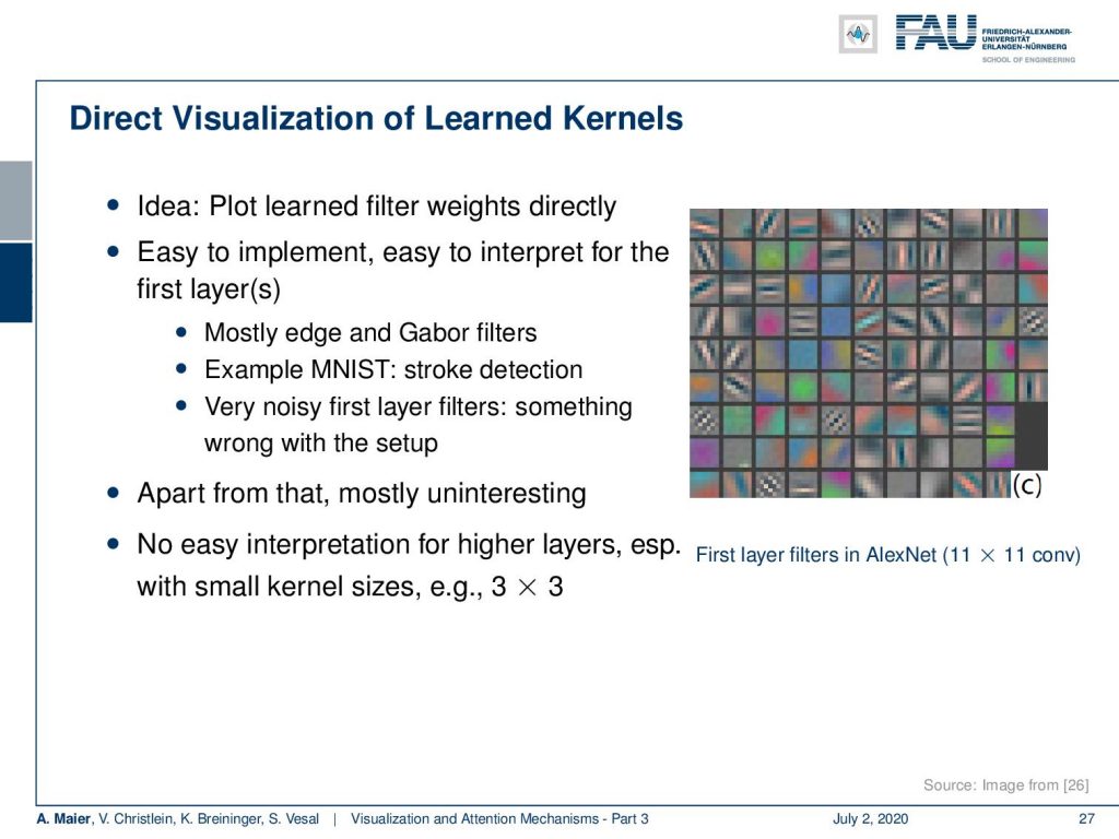
So, the idea is that you can plot the learned filter weights directly. It’s easy to implement. It’s also easy to interpret for the first layer. Here, you see some examples of the first layer filters in AlexNet. If you see very noisy first layers, then you can probably already guess that there’s something wrong. So, for example, you’re picking up the noise characteristic of a specific sensor. Apart from that, it’s mostly uninteresting because you can see that they take the shape of edge and Gabor filters, but it doesn’t tell you really what’s happening in later parts of the network. If you have small kernels, then you can probably still interpret them. But if you go deeper you would have to understand what’s already happened in the first layers. So, they somehow stack and you can’t understand what’s really happening inside the deeper layers.
So, we need some different ideas. One idea is that we visualize the activations. The kernels are difficult to interpret. So, we look at the activations that are generated by the Kernels because they tell us what the network is computing from a specific input. If you have a strong response, it probably means that the feature is present. If you have a weaker response, the feature is probably absent.
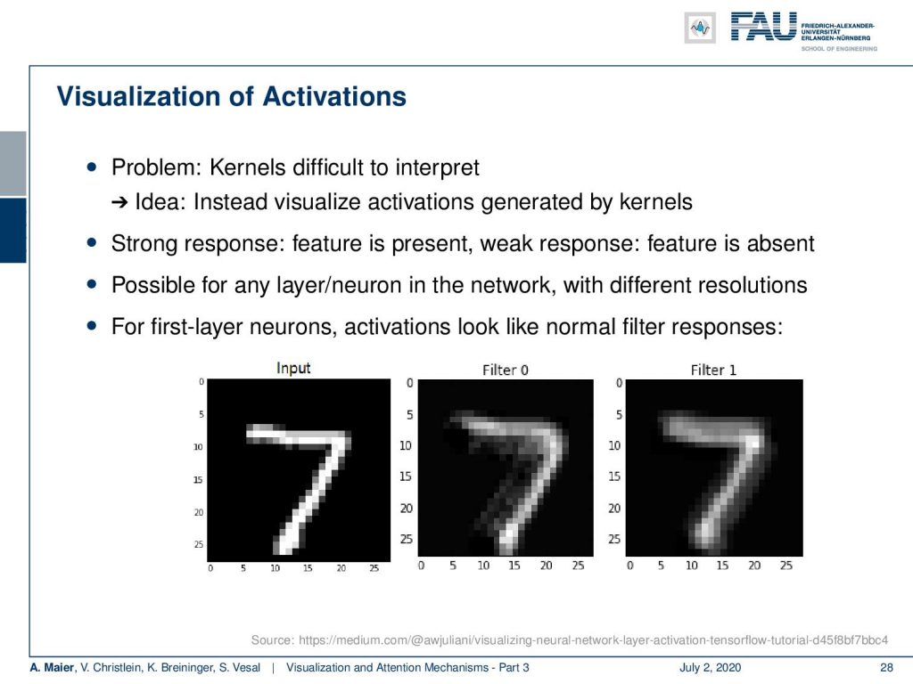
So, how does this look like? For the first, layer you can see that the activations then look like normal filter responses. So, you see here the input and then filter zero and for the one, you can see that they somehow filter the input. Of course, you can then proceed and look at the activations of deeper layers. Then, you already realized that looking at the activations maybe somehow interesting, but the activation maps typically lose resolution very quickly due to the downsampling. So, this means that you then result in very coarse activation maps.
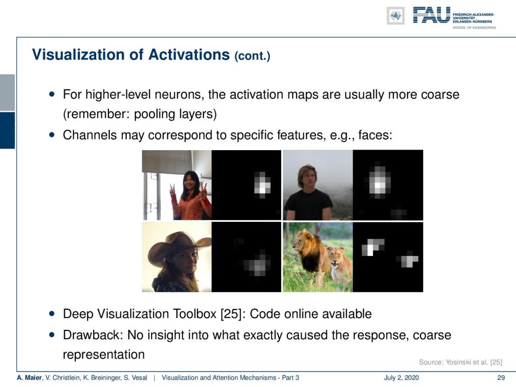
So here, you see a visualization that may correspond to face detection or face-like features. Then, we can start speculating what this kind of feature is actually representing inside the deep network. There’s the deep visualization toolbox that I have in [25] and it’s online available. It allows you to compute things like that. Well, the drawback is, of course, that we don’t get precise information, why that specific neuron was activated or why this feature map takes this shape.
Well, what else can we do? We can investigate features via occlusion. The idea here is that you move a masking patch around the input image. With this patch then you kind of remove information from the image. Then, you try to visualize the confidence for a specific decision with respect to the different positions of this occluding patch.
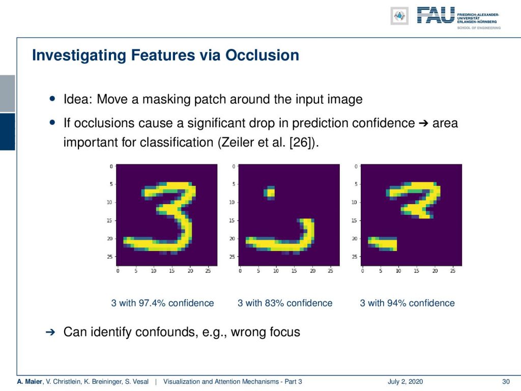
Then, of course, an area where the patch caused a large drop in confidence is probably an area that is related to the specific classification. So, we have some examples here. We have this patch to mask the original input on the left. The two different versions of masking are in the center and on the right. Then, you can see that the reduction in confidence for the number three is much larger in the center image than on the right-hand side image. So, we can try to identify confounds or wrong focus using this kind of technique.
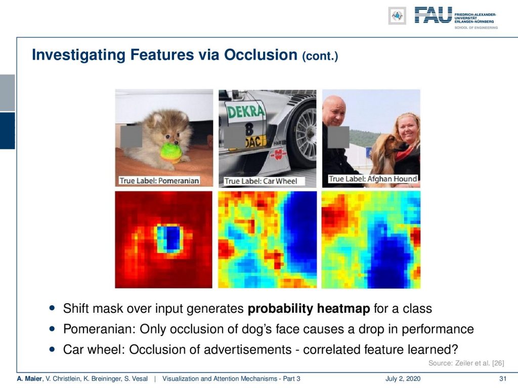
Let’s look at some more examples. Here, you see the pomeranian image on the top left. The important part of the image is really located in the center. If you start occluding the center, also the confidence for the class pomeranian will go down. In the middle column, you see the true label car wheel and the recorded image. On the bottom, you can see that if you hide the car wheel then, of course, the confidence drops. But if you start hiding parts of the advertisements on the car, also the confidence drops. So, this is a kind of confounder that was probably learned. A car wheel may be in close collocation to such other parts of the image even including advertisements. Here on the right, you see the true label Afghan hound. If you start occluding the dog, of course, the confidence actually breaks down. The person on the top left for example is completely unrelated. But covering the face of the owner or seeming owner also causes a reduction in the confidence. So you might argue that dog owners start to become similar to their dogs. No, this is also a confounder!
Well, let’s look into a third technique. Here, we want to find the maximal activations of specific layers or neurons. The idea here is that we just look at the patches that have been shown to a network and we order them by activation in a specific neuron.
What you can then generate are sequences like this one. So, you see that this specific neuron has been activated with 0.1, 0.9, 0.9, 0.8, 0.8, and you can see these were the patches that were maximally activating this neuron. So, you could argue: “Well, it’s a god face detector, or is it a dark sport detector.”
So, you could very easily figure out what “false friends” are. This is comparatively easy to find, but the drawback is of course that you don’t necessarily get a semantic meaning. You could argue that these forms are the base vectors of representation. Here, we have another example and you could say “Well, what kind of detector is? This is a red flower and tomato sauce detector. Or is this a detector for specular highlights?” Well, at least you can figure out which neuron is related to what kind of input. So, you kind of get some feeling what’s happening in the network and which things cluster together.
Speaking of clustering: Then you can also actually use the clustering of inputs to visualize how similar different inputs are for a specific deep network. This leads to the T stochastic neighborhood embedding visualization technique.
Now here, the idea is that you compute the activations of the last layer and group the inputs with respect to their similarity in the last layer activation. So, you essentially perform dimensionality of the last layer activations. These are the ones that are relevant for the classification and are likely to encode the feature representation of your trained network. Then, you actually perform this dimensionality reduction technique and produce a 2-D map.
This allows you to see what your network thinks are similar inputs. So, this is, of course, an embedding of a very high dimensional space in 2-D. There’s, of course, a lot of loss of information. If you do this, still the technique is very interesting. If I zoom in into different parts here, you can see that we actually form clusters of different categories in this kind of dimensionality reduction. So, you can see that images that are perceived similarly by the neural network are also located in a direct neighborhood. The dimensionality reduction that we do reveals the internal representations. Actually, if you look at those neighborhoods, they kind of make sense. So, this is actually something that helps us to understand and develop confidence in the feature extraction that our deep neural network is doing.
None of the presented techniques so far was really satisfying. So, next time in deep learning, we want to talk about more visualization methods. In particular, we want to look into gradient-based procedures. So, we want to use a kind of backpropagation-type idea in order to create visualizations. Other interesting approaches are optimization-based techniques. Here, we are actually very close to what we’ve already seen in the adversarial examples. So, thank you very much for listening and see you in the next video. Bye-bye!
If you liked this post, you can find more essays here, more educational material on Machine Learning here, or have a look at our Deep LearningLecture. I would also appreciate a follow on YouTube, Twitter, Facebook, or LinkedIn in case you want to be informed about more essays, videos, and research in the future. This article is released under the Creative Commons 4.0 Attribution License and can be reprinted and modified if referenced. If you are interested in generating transcripts from video lectures try AutoBlog.
Links
Yosinski et al.: Deep Visualization Toolbox
Olah et al.: Feature Visualization
Adam Harley: MNIST Demo
References
[1] Dzmitry Bahdanau, Kyunghyun Cho, and Yoshua Bengio. “Neural Machine Translation by Jointly Learning to Align and Translate”. In: 3rd International Conference on Learning Representations, ICLR 2015, San Diego, 2015.
[2] T. B. Brown, D. Mané, A. Roy, et al. “Adversarial Patch”. In: ArXiv e-prints (Dec. 2017). arXiv: 1712.09665 [cs.CV].
[3] Jianpeng Cheng, Li Dong, and Mirella Lapata. “Long Short-Term Memory-Networks for Machine Reading”. In: CoRR abs/1601.06733 (2016). arXiv: 1601.06733.
[4] Jacob Devlin, Ming-Wei Chang, Kenton Lee, et al. “BERT: Pre-training of Deep Bidirectional Transformers for Language Understanding”. In: CoRR abs/1810.04805 (2018). arXiv: 1810.04805.
[5] Neil Frazer. Neural Network Follies. 1998. URL: https://neil.fraser.name/writing/tank/ (visited on 01/07/2018).
[6] Ross B. Girshick, Jeff Donahue, Trevor Darrell, et al. “Rich feature hierarchies for accurate object detection and semantic segmentation”. In: CoRR abs/1311.2524 (2013). arXiv: 1311.2524.
[7] Alex Graves, Greg Wayne, and Ivo Danihelka. “Neural Turing Machines”. In: CoRR abs/1410.5401 (2014). arXiv: 1410.5401.
[8] Karol Gregor, Ivo Danihelka, Alex Graves, et al. “DRAW: A Recurrent Neural Network For Image Generation”. In: Proceedings of the 32nd International Conference on Machine Learning. Vol. 37. Proceedings of Machine Learning Research. Lille, France: PMLR, July 2015, pp. 1462–1471.
[9] Nal Kalchbrenner, Lasse Espeholt, Karen Simonyan, et al. “Neural Machine Translation in Linear Time”. In: CoRR abs/1610.10099 (2016). arXiv: 1610.10099.
[10] L. N. Kanal and N. C. Randall. “Recognition System Design by Statistical Analysis”. In: Proceedings of the 1964 19th ACM National Conference. ACM ’64. New York, NY, USA: ACM, 1964, pp. 42.501–42.5020.
[11] Andrej Karpathy. t-SNE visualization of CNN codes. URL: http://cs.stanford.edu/people/karpathy/cnnembed/ (visited on 01/07/2018).
[12] Alex Krizhevsky, Ilya Sutskever, and Geoffrey E Hinton. “ImageNet Classification with Deep Convolutional Neural Networks”. In: Advances In Neural Information Processing Systems 25. Curran Associates, Inc., 2012, pp. 1097–1105. arXiv: 1102.0183.
[13] Thang Luong, Hieu Pham, and Christopher D. Manning. “Effective Approaches to Attention-based Neural Machine Translation”. In: Proceedings of the 2015 Conference on Empirical Methods in Natural Language Lisbon, Portugal: Association for Computational Linguistics, Sept. 2015, pp. 1412–1421.
[14] A. Mahendran and A. Vedaldi. “Understanding deep image representations by inverting them”. In: 2015 IEEE Conference on Computer Vision and Pattern Recognition (CVPR). June 2015, pp. 5188–5196.
[15] Andreas Maier, Stefan Wenhardt, Tino Haderlein, et al. “A Microphone-independent Visualization Technique for Speech Disorders”. In: Proceedings of the 10th Annual Conference of the International Speech Communication Brighton, England, 2009, pp. 951–954.
[16] Volodymyr Mnih, Nicolas Heess, Alex Graves, et al. “Recurrent Models of Visual Attention”. In: CoRR abs/1406.6247 (2014). arXiv: 1406.6247.
[17] Chris Olah, Alexander Mordvintsev, and Ludwig Schubert. “Feature Visualization”. In: Distill (2017). https://distill.pub/2017/feature-visualization.
[18] Prajit Ramachandran, Niki Parmar, Ashish Vaswani, et al. “Stand-Alone Self-Attention in Vision Models”. In: arXiv e-prints, arXiv:1906.05909 (June 2019), arXiv:1906.05909. arXiv: 1906.05909 [cs.CV].
[19] Mahmood Sharif, Sruti Bhagavatula, Lujo Bauer, et al. “Accessorize to a Crime: Real and Stealthy Attacks on State-of-the-Art Face Recognition”. In: Proceedings of the 2016 ACM SIGSAC Conference on Computer and Communications CCS ’16. Vienna, Austria: ACM, 2016, pp. 1528–1540. A.
[20] K. Simonyan, A. Vedaldi, and A. Zisserman. “Deep Inside Convolutional Networks: Visualising Image Classification Models and Saliency Maps”. In: International Conference on Learning Representations (ICLR) (workshop track). 2014.
[21] J.T. Springenberg, A. Dosovitskiy, T. Brox, et al. “Striving for Simplicity: The All Convolutional Net”. In: International Conference on Learning Representations (ICRL) (workshop track). 2015.
[22] Dmitry Ulyanov, Andrea Vedaldi, and Victor S. Lempitsky. “Deep Image Prior”. In: CoRR abs/1711.10925 (2017). arXiv: 1711.10925.
[23] Ashish Vaswani, Noam Shazeer, Niki Parmar, et al. “Attention Is All You Need”. In: CoRR abs/1706.03762 (2017). arXiv: 1706.03762.
[24] Kelvin Xu, Jimmy Ba, Ryan Kiros, et al. “Show, Attend and Tell: Neural Image Caption Generation with Visual Attention”. In: CoRR abs/1502.03044 (2015). arXiv: 1502.03044.
[25] Jason Yosinski, Jeff Clune, Anh Mai Nguyen, et al. “Understanding Neural Networks Through Deep Visualization”. In: CoRR abs/1506.06579 (2015). arXiv: 1506.06579.
[26] Matthew D. Zeiler and Rob Fergus. “Visualizing and Understanding Convolutional Networks”. In: Computer Vision – ECCV 2014: 13th European Conference, Zurich, Switzerland, Cham: Springer International Publishing, 2014, pp. 818–833.
[27] Han Zhang, Ian Goodfellow, Dimitris Metaxas, et al. “Self-Attention Generative Adversarial Networks”. In: Proceedings of the 36th International Conference on Machine Learning. Vol. 97. Proceedings of Machine Learning Research. Long Beach, California, USA: PMLR, Sept. 2019, pp. 7354–7363. A.