Lecture Notes in Deep Learning: Visualization & Attention – Part 4

Gradient and Optimisation-based Methods

These are the lecture notes for FAU’s YouTube Lecture “Deep Learning“. This is a full transcript of the lecture video & matching slides. We hope, you enjoy this as much as the videos. Of course, this transcript was created with deep learning techniques largely automatically and only minor manual modifications were performed. Try it yourself! If you spot mistakes, please let us know!

Welcome back to deep learning! Today, we want to look a bit more into visualization techniques and in particular, the gradient-based and optimization-based procedures.

Okay, so let’s see what I’ve got for you. Let’s talk first about the gradient-based visualizations and here the idea is that we want to figure out which input pixel is most significant to a neuron.

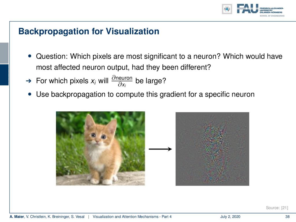
If we would change it, what would cause a large variation in the actual output of our neural network? What we actually want to compute is the partial derivative of the neuron under consideration, maybe for an output neuron-like for the class “cat”. Then, we want to compute the partial derivative with respect to the input. This is essentially backpropagation through the entire network. Then, we can visualize this gradient as a type of image which we have been doing here for the cat image. You can see that, of course, this is a color gradient. You see that this is a bit of a noisy image but you can see that what is related to class “cat”, here is obviously also located in the area where the cat is in the image.

We will learn several different approaches to do this. The first one is based on [20]. For backpropagation, we actually need a loss of what we want to backpropagate. We simply take a pseudo loss that is the activation of an arbitrary neuron or layer. Typically, what you want to do is you want to take neurons in the output layer because they can be associated with a class.

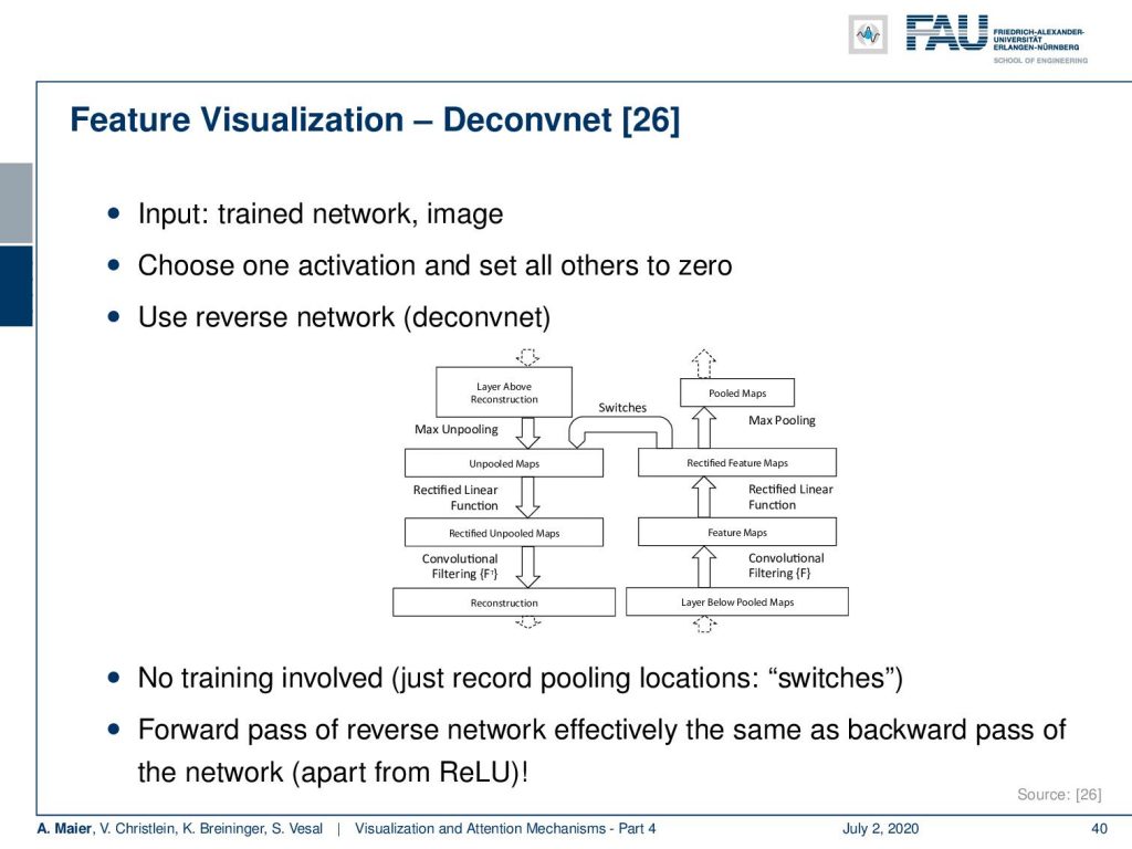
What you can also do is instead of using backpropagation, you can build a nearly equivalent alternative which uses a kind of reverse network. This is the Deconvnet from [26]. So here, the input is the trained network and some image. Then, you choose one activation and set all of the other activations to zero. Next, you build a reverse network and you can see the idea here that this is essentially containing the same as the network but just in reverse sequence with so-called unpooling steps. Now, with these unpooling steps and the reverse computation, you can see that we can also produce a kind of gradient estimate. The nice thing about this one is, there’s no training involved. So, you just have to record the pooling location in the switches and the forward path of the reverse Network. Effectively this is the same as the backward-pass of the network apart from the rectified linear units which we’ll look at in a couple of slides.

Here, we show the visualizations of the top nine activations, the gradient, and the corresponding patch. So for example, you can reveal with this one that this kind of feature map seems to focus on green patchy areas. You could argue that this is more a kind of background feature that tries to detect grass patches in the image.

So, what else? Well, there’s guided backpropagation. Guided backpropagation is a very similar concept. The idea here is that you want to find positively correlated features. So we are looking for positive gradients because we assume that the features that are positive are the ones that the neuron is interested in. The negative gradients are the ones that the neuron is not interested in.

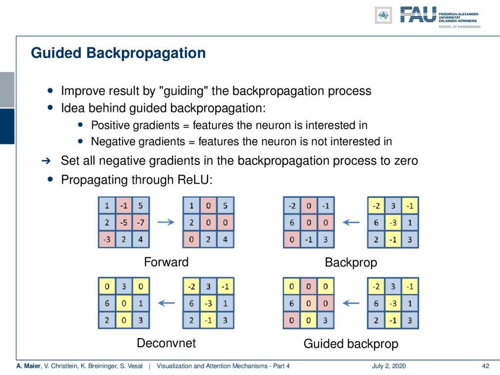
So, the idea is then to set all negative gradients in the backpropagation to zero. We can show you now the different processes of the ReLU during the forward and backward passes with the different kinds of gradient backpropagation techniques. Well, of course, if you have these input activations, then in the forward pass in the ReLU, you would simply cancel out all the negative values and set them to zero. Now, what happens in the backpropagation for the three different alternatives? Let’s look at what the typical backpropagation does and note that we show here the negative entries that came from the sensitivity in yellow. If you now try to backpropagate this, you have to remember which entries in the forward pass were negative and you set those values again to zero. You keep everything that came from the sensitivity of the previous layer in order to do so. Now if you do Deconvnet, you don’t need to remember the switches from the forward-pass, but you set all the entries that are negative in the sensitivity to zero and backpropagate. This way now, the guided backpropagation actually does both. So it remembers the forward-pass and sets all of those elements to zero. It sets all of the elements of the sensitivities to zero. So, it’s essentially a union of backpropagation and Deconvnet in terms of canceling negative values. You can see that the guided backpropagation only keeps very little sensitivity throughout the entire backpropagation process.

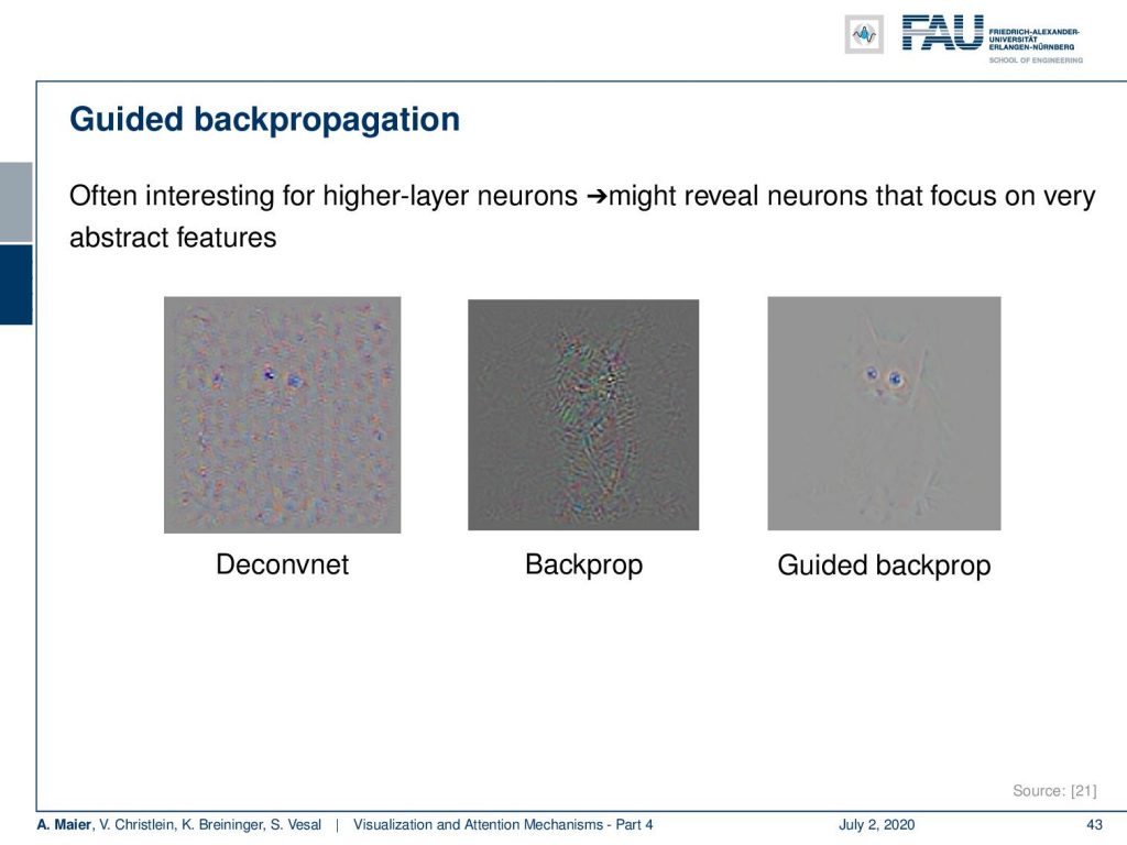
Now let’s look at the comparison of the different gradients. One thing that you can see is that in Deconvnet, we get pretty noisy activations and backpropagation. We can see that we at least focus on the object of interest and the guided backpropagation has a very sparse representation but you can very clearly see even in this gradient image, the most important features like the eyes of the cat and so on. So, this is a very nice way that might help you reveal which neurons focus on what activity in that specific input.

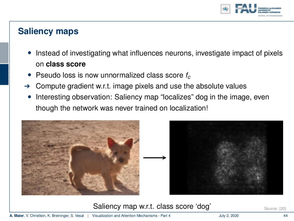
This then finally leads to saliency maps. Here, you don’t want to investigate what influences two neurons but you want to investigate the impact of pixels on a class “dog”. So now, you take the pseudo loss as an unnormalized task, compute the gradient with respect to the image pixels, and use absolute values. Then, the interesting observation that we make with this is that it kind of produces a saliency map that localizes the dog in the image, even though the network was never trained on localization. So, this is a very interesting approach that can help you to identify where the decisive information is actually located in the image.

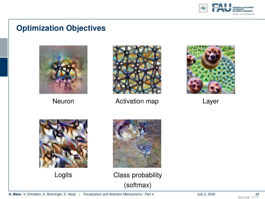
What else can be done? Well, there’s parameter visualization based on optimization. Now, the idea is that we want to go towards different levels. So, if we want to optimize with respect to a neuron, to an activation map, a layer, the actual logits, or the class probability which is essentially the softmax function, we take them as pseudo loss in order to create optimal inputs.

We’ve already seen something very similar in the first video where we had this example from DeepDream. Inceptionism is essentially doing something very similar. It takes some input and then it alters the input such that different neurons are maximally activated.

There you can see that these neurons somehow encode specific parts of animals or things that it likes to recognize. If you now maximize the input with respect to that particular neuron, you can see that then the shapes that it likes start to appear in this image. So, the idea is that you change the input such that the neuron is maximally activated. So, we are essentially not just computing the gradient up to the image, but we are also actively changing the image with respect to that particular or layer, softmax, or output. The original idea for this was, of course, visualization.

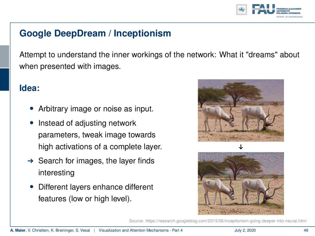
So, you try to understand the inner workings of the networks by dreaming about when presented with images. You start with the image or even noise as input. Then, you adjust the image towards maximizing activations in a complete layer. For different layers, it highlights different things in the image. So, we can create this kind of Inceptionism. If you activate mostly early layers, you see that the image content is not that much changed but you create those brush and stroke-like appearances in the images.

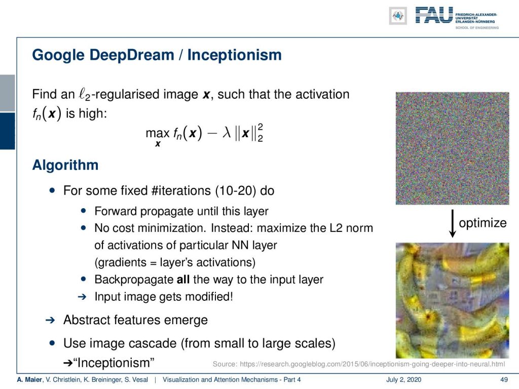
Now you can even go ahead and start this with random input. Then it’s not just optimizing the input with respect to a specific output. You need some additional regularization. We can show this here in this small formula. So, we are now taking some input x which is a random image. We feed it into our network and a specific neuron or output neuron. Then, we maximize the activation and we add a regularization. This regularizer punishes if our x deviates from a specific norm. What is used in this example, it’s simply the L2 norm. Later, we will also see that maybe also other norms may be suitable for this. So, you start with this noise input that we show on the top right. Then, you optimize until you find a maximum activation for that specific neuron or layer. At the same time, you postulate that your input image somehow has to be smooth because otherwise, you be generating these very, very noisy images. They are not so nice for interpretation and of course, the bottom right image shows you some kind of structures that you know can interpret. So, you see these abstract features emerging and then you can use this as a kind of cascade from small to large scales and this produces the so-called inceptionism.

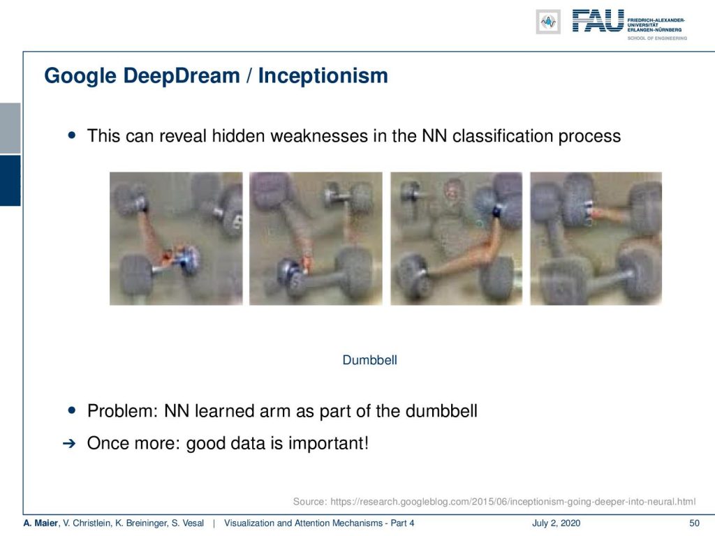
Here, we can use that for example to reveal hidden weaknesses in the neural network classification process. Here, we see different realizations for the class “dumbbell”. You can see, it’s not only the dumbbell that is shown in the image, but it is also recreating the arm that is holding the dumbbell. So, we can see here that correlated things are kind of learned, when they have been presented to the network. So, we kind of can figure out what the memory of that specific class or neuron with respect to the input is. So, again we learned once more good data is really important.

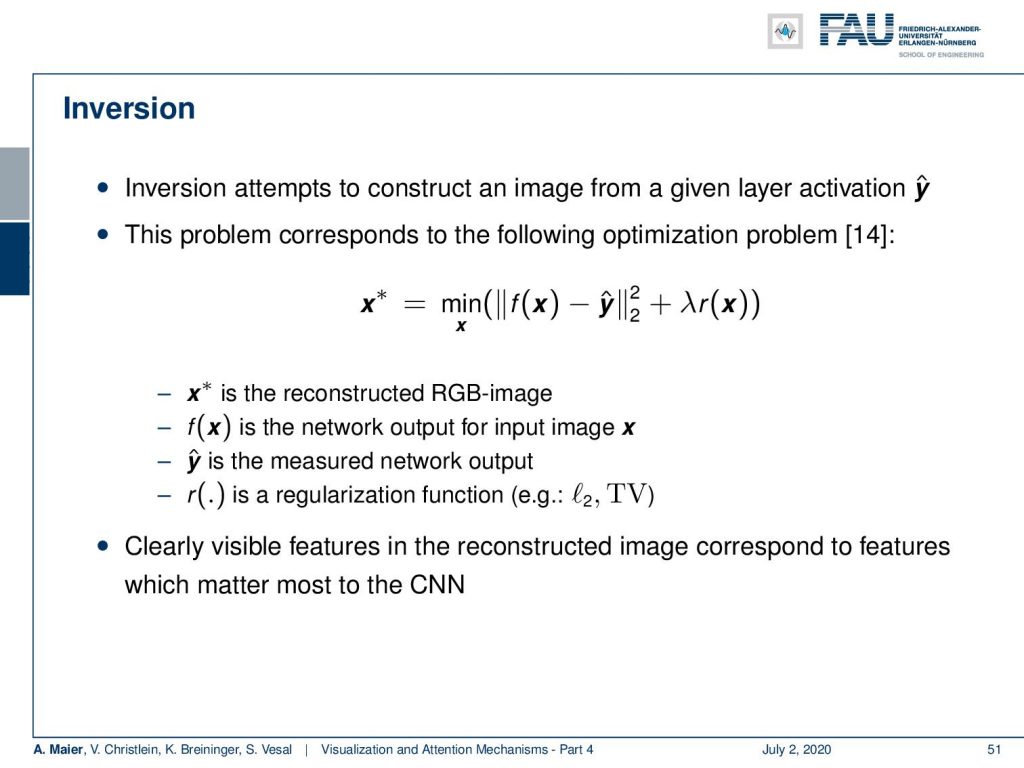
This actually leads us to another step that we could do in order to figure out what’s happening inside of the neural network. These are inversion techniques and here the idea is very similar to what we’ve seen in the inceptionism idea. But now, we actually want to invert from the activation what was the actual input. What you hear quite frequently, for example, as security measures to anonymize data: “Let’s just take the activations of Layer 5 and discard all the previous activations and inputs. We just store the Layer 5 activations because there is no way how I can reconstruct the original image if I only know that Layer 5 activation.”

Now with inversion, if you know the network, its processes, and the specific activations for a specific layer, then you can try to reconstruct what the actual input was. So again, we have the output of our network in that particular layer. So let’s say f(x) is the output of a layer and we have y hat. Now, y hat is the measured network’s output or the measured layer activation. So, we have the Layer 5 activation and we don’t know what the input x is. So, we are looking for x and we try to minimize this function such that we find with an x to best match that specific activation.

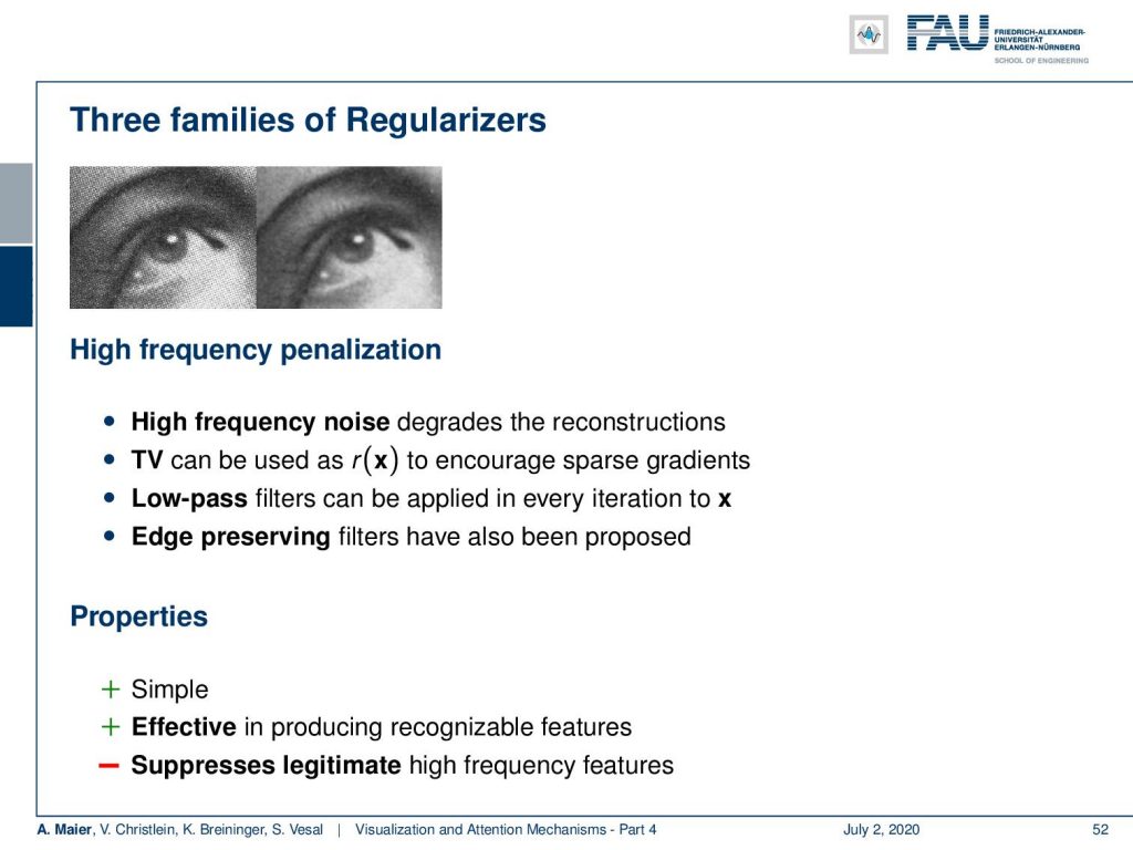
This is a classical inverse problem. You add in order to get a more stable output, an additional regularizer λ times R(x). This regularizer is something that is very important. So, the regularizer stabilizes the inversion and there are very common techniques for regularization that use specific properties of natural images in order to create something that is likely a natural image. So, of course, high-frequency noise would degrade the reconstructions. This is why we are using this additional L2 norm in order to prevent the appearance of noise in the created images. In addition to that, you can also use the so-called total variation. We know that natural images typically have sparse gradients and total variation is a minimization technique that enforces your image to have a very low number of gradients. Gradients are essentially edges and in a typical image, there are only a few edge pixels and many more homogeneous areas. So, TV minimization produces images with few edges and, of course, also a little noise. It specifically also allows high piecewise constant jumps like in real edges. Of course, you could also work with low-pass and other edge-preserving filters. A classic one is the wavelet regularization. So this is simple, it’s effective and, of course, it will also suppress real edges and other high-frequency information.

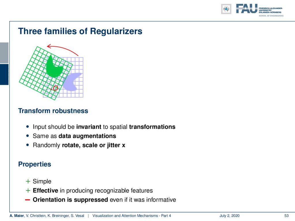
Well, what else can be done? You can also use other regularizers like transform robustness. So, the input should actually be invariant to special transformation. So this is similar to data augmentation and therefore, you can randomly rotate, scale, or jitter x. So, this is also very simple and it’s effective in producing recognizable features. Often the orientation is suppressed even if it was informative. So, we have to be careful about that.

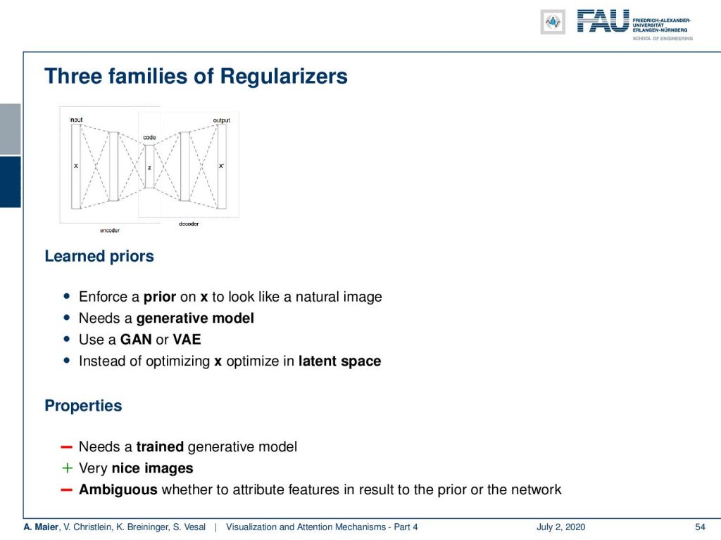
A last kind of regularizer that is very common is that you have learned priors. So, for example, you can use a train network and say “I want to have a specific distribution in layer #4.” Then, I try to generate images that have a very similar characteristic. Here, instead of optimizing with respect to a specific norm that we know that is useful, we assume that the representations that are produced in a specific layer are useful in order to measure the content of the image. Then, you can actually use this as a kind of regularizer to produce images. So of course, you need a trained generative model if you want to use things like this. This produces very nice images, but it may be ambiguous because parts of what you introduce into the results stem from the pre-trained network. So, you have to see this with a bit of caution.

So, let’s look at some examples [14] actually generated images by inversion. This is pretty impressive. Again, this is an AlexNet-type of network and here you have the input and then the inversion:

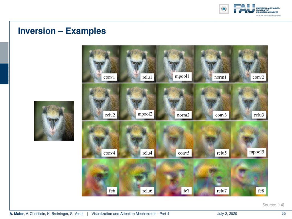
At the conv layer 1, you can see we can almost exactly reproduce the image. After ReLu 1 not much changed. Pooling – no big effect. Then, the second layer, and so on. You can see that up to convolution layer #4, we are very close to the true input. This has undergone several steps of pooling already and still, we are able to reproduce the input very closely to the original input. Very interesting! Then, you see that I really have to go towards – let’s say – Layer 6 or Layer 7, until I reach a point where it becomes impossible or close to impossible to guess what the original input was. So only, from Layer 6/Layer 7, we start deviating significantly from the original input. Still until Layer 5, we can reconstruct quite well what the original input is. So, if anybody tells you that they want to anonymize data by cutting off the first two layers, then you see that with these inversion techniques this is maybe not such a great idea. It’s not unlikely that you will be able to reconstruct the original input only by means of seeing the activations and the network structure.

Okay. So next time, we want to talk about a second topic that is somewhat related to visualization. We want to talk about attention and attention mechanisms. You’ve already seen that with the visualization techniques, we can somehow figure out which pixels are related to what kind of classification. Now, we want to spin this a little further and use this to guide the focus of the attention of the network towards specific areas. So, this will also be a very interesting video. Looking forward to seeing you in the next video. Bye-bye!

If you liked this post, you can find more essays here, more educational material on Machine Learning here, or have a look at our Deep LearningLecture. I would also appreciate a follow on YouTube, Twitter, Facebook, or LinkedIn in case you want to be informed about more essays, videos, and research in the future. This article is released under the Creative Commons 4.0 Attribution License and can be reprinted and modified if referenced. If you are interested in generating transcripts from video lectures try AutoBlog.

Links

Yosinski et al.: Deep Visualization Toolbox
Olah et al.: Feature Visualization
Adam Harley: MNIST Demo

References

[1] Dzmitry Bahdanau, Kyunghyun Cho, and Yoshua Bengio. “Neural Machine Translation by Jointly Learning to Align and Translate”. In: 3rd International Conference on Learning Representations, ICLR 2015, San Diego, 2015.
[2] T. B. Brown, D. Mané, A. Roy, et al. “Adversarial Patch”. In: ArXiv e-prints (Dec. 2017). arXiv: 1712.09665 [cs.CV].
[3] Jianpeng Cheng, Li Dong, and Mirella Lapata. “Long Short-Term Memory-Networks for Machine Reading”. In: CoRR abs/1601.06733 (2016). arXiv: 1601.06733.
[4] Jacob Devlin, Ming-Wei Chang, Kenton Lee, et al. “BERT: Pre-training of Deep Bidirectional Transformers for Language Understanding”. In: CoRR abs/1810.04805 (2018). arXiv: 1810.04805.
[5] Neil Frazer. Neural Network Follies. 1998. URL: https://neil.fraser.name/writing/tank/ (visited on 01/07/2018).
[6] Ross B. Girshick, Jeff Donahue, Trevor Darrell, et al. “Rich feature hierarchies for accurate object detection and semantic segmentation”. In: CoRR abs/1311.2524 (2013). arXiv: 1311.2524.
[7] Alex Graves, Greg Wayne, and Ivo Danihelka. “Neural Turing Machines”. In: CoRR abs/1410.5401 (2014). arXiv: 1410.5401.
[8] Karol Gregor, Ivo Danihelka, Alex Graves, et al. “DRAW: A Recurrent Neural Network For Image Generation”. In: Proceedings of the 32nd International Conference on Machine Learning. Vol. 37. Proceedings of Machine Learning Research. Lille, France: PMLR, July 2015, pp. 1462–1471.
[9] Nal Kalchbrenner, Lasse Espeholt, Karen Simonyan, et al. “Neural Machine Translation in Linear Time”. In: CoRR abs/1610.10099 (2016). arXiv: 1610.10099.
[10] L. N. Kanal and N. C. Randall. “Recognition System Design by Statistical Analysis”. In: Proceedings of the 1964 19th ACM National Conference. ACM ’64. New York, NY, USA: ACM, 1964, pp. 42.501–42.5020.
[11] Andrej Karpathy. t-SNE visualization of CNN codes. URL: http://cs.stanford.edu/people/karpathy/cnnembed/ (visited on 01/07/2018).
[12] Alex Krizhevsky, Ilya Sutskever, and Geoffrey E Hinton. “ImageNet Classification with Deep Convolutional Neural Networks”. In: Advances In Neural Information Processing Systems 25. Curran Associates, Inc., 2012, pp. 1097–1105. arXiv: 1102.0183.
[13] Thang Luong, Hieu Pham, and Christopher D. Manning. “Effective Approaches to Attention-based Neural Machine Translation”. In: Proceedings of the 2015 Conference on Empirical Methods in Natural Language Lisbon, Portugal: Association for Computational Linguistics, Sept. 2015, pp. 1412–1421.
[14] A. Mahendran and A. Vedaldi. “Understanding deep image representations by inverting them”. In: 2015 IEEE Conference on Computer Vision and Pattern Recognition (CVPR). June 2015, pp. 5188–5196.
[15] Andreas Maier, Stefan Wenhardt, Tino Haderlein, et al. “A Microphone-independent Visualization Technique for Speech Disorders”. In: Proceedings of the 10th Annual Conference of the International Speech Communication Brighton, England, 2009, pp. 951–954.
[16] Volodymyr Mnih, Nicolas Heess, Alex Graves, et al. “Recurrent Models of Visual Attention”. In: CoRR abs/1406.6247 (2014). arXiv: 1406.6247.
[17] Chris Olah, Alexander Mordvintsev, and Ludwig Schubert. “Feature Visualization”. In: Distill (2017). https://distill.pub/2017/feature-visualization.
[18] Prajit Ramachandran, Niki Parmar, Ashish Vaswani, et al. “Stand-Alone Self-Attention in Vision Models”. In: arXiv e-prints, arXiv:1906.05909 (June 2019), arXiv:1906.05909. arXiv: 1906.05909 [cs.CV].
[19] Mahmood Sharif, Sruti Bhagavatula, Lujo Bauer, et al. “Accessorize to a Crime: Real and Stealthy Attacks on State-of-the-Art Face Recognition”. In: Proceedings of the 2016 ACM SIGSAC Conference on Computer and Communications CCS ’16. Vienna, Austria: ACM, 2016, pp. 1528–1540. A.
[20] K. Simonyan, A. Vedaldi, and A. Zisserman. “Deep Inside Convolutional Networks: Visualising Image Classification Models and Saliency Maps”. In: International Conference on Learning Representations (ICLR) (workshop track). 2014.
[21] J.T. Springenberg, A. Dosovitskiy, T. Brox, et al. “Striving for Simplicity: The All Convolutional Net”. In: International Conference on Learning Representations (ICRL) (workshop track). 2015.
[22] Dmitry Ulyanov, Andrea Vedaldi, and Victor S. Lempitsky. “Deep Image Prior”. In: CoRR abs/1711.10925 (2017). arXiv: 1711.10925.
[23] Ashish Vaswani, Noam Shazeer, Niki Parmar, et al. “Attention Is All You Need”. In: CoRR abs/1706.03762 (2017). arXiv: 1706.03762.
[24] Kelvin Xu, Jimmy Ba, Ryan Kiros, et al. “Show, Attend and Tell: Neural Image Caption Generation with Visual Attention”. In: CoRR abs/1502.03044 (2015). arXiv: 1502.03044.
[25] Jason Yosinski, Jeff Clune, Anh Mai Nguyen, et al. “Understanding Neural Networks Through Deep Visualization”. In: CoRR abs/1506.06579 (2015). arXiv: 1506.06579.
[26] Matthew D. Zeiler and Rob Fergus. “Visualizing and Understanding Convolutional Networks”. In: Computer Vision – ECCV 2014: 13th European Conference, Zurich, Switzerland, Cham: Springer International Publishing, 2014, pp. 818–833.
[27] Han Zhang, Ian Goodfellow, Dimitris Metaxas, et al. “Self-Attention Generative Adversarial Networks”. In: Proceedings of the 36th International Conference on Machine Learning. Vol. 97. Proceedings of Machine Learning Research. Long Beach, California, USA: PMLR, Sept. 2019, pp. 7354–7363. A.

Category: Lecture Notes in Deep Learning