Lecture Notes in Pattern Recognition: Episode 26 – Mercer’s Theorem and the Kernel SVM

These are the lecture notes for FAU’s YouTube Lecture “Pattern Recognition“. This is a full transcript of the lecture video & matching slides. We hope, you enjoy this as much as the videos. Of course, this transcript was created with deep learning techniques largely automatically and only minor manual modifications were performed. Try it yourself! If you spot mistakes, please let us know!

Welcome back everybody to Pattern Recognition! Today we want to explore a bit more the concept of kernels. We will look into something that is called Mercer’s Theorem. Looking forward to exploring kernel spaces!

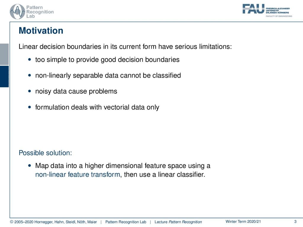
Let’s have a look into kernels! So far we’ve seen that the linear decision boundaries in their current form have serious limitations. It’s too simple to provide good decision boundaries. Nonlinearly separable data cannot be classified. Noisy data cause problems, and also this formulation allows you to work with vectorial data only. So one possible solution that we already hinted at is mapping into a higher-dimensional space using a non-linear feature transform and then use a linear classifier.

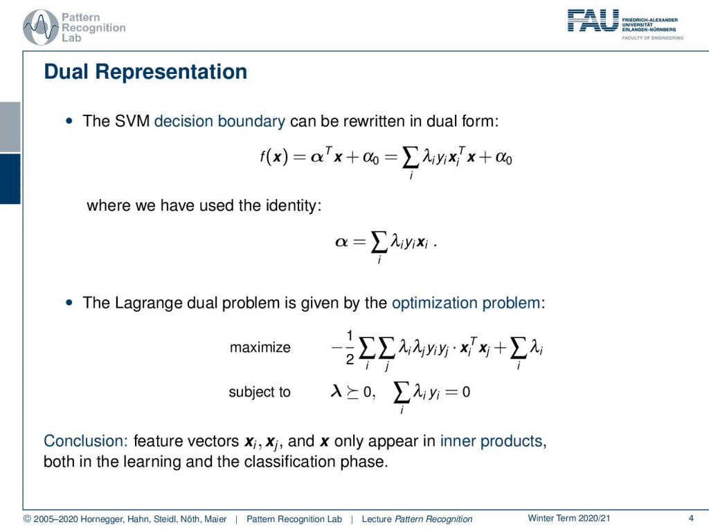
We’ve seen that the SVM decision boundary can be rewritten in dual form. Then we could see that we essentially got rid of the actual normal vector and everything could be written as a sum over the Lagrange multipliers, the class observations, and the extra features. And in this particular optimization problem, we’ve seen that the feature vectors only appear as inner products. So the conclusion is that we only have inner products here, so this can be applied in both the learning and the classification phase.

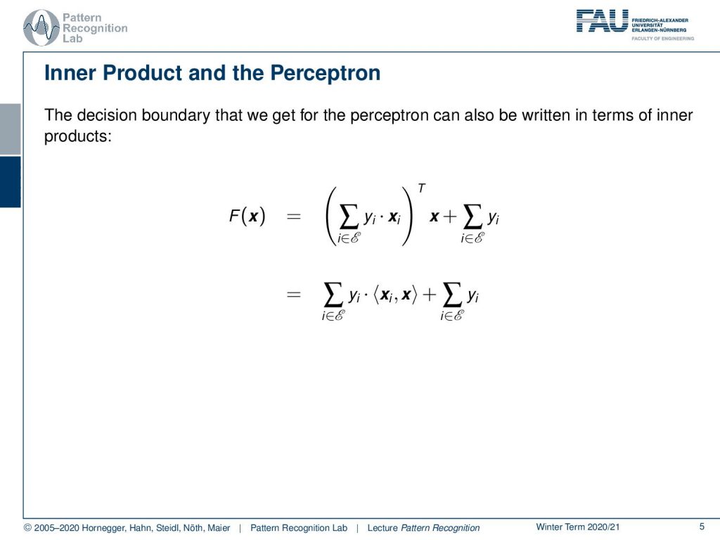
Now let’s look again at this inner product in a bit more detail. We’ve seen that this was also the case in the perceptron. There we’ve seen that essentially, we were summing up over all the steps during the training procedure. And we already have seen that also in this case we essentially only had inner products for the decision boundary. Also, we’ve seen that we only need two observations that produced updates of our decision boundary during the training process. This is the set ℰ here if you remember. So again, everything can be brought down to inner products.

We can use feature transforms now. This feature transform Φ is mapping from d-dimensional to D-dimensional space. And now the capital D is larger or equal to d, such that the resulting features are linearly separable. Let’s look into one example. Here we have some original feature space that is centered around 0. All the observations from one class are in the center and all the observations from the outer class are outside a line. It is very clear that this example cannot be solved with a linear decision boundary. But now I take the feature transform Φ = (x₁²,x₂²)^T. So this has exactly the same dimensionality. And what we see is by mapping onto essentially the square dimensions we can now find a linear decision boundary. Now, this is a simple example. It may be more difficult.

And it already gets difficult if we start using data that is not centered. In this case, if we apply our feature transform we see that we, unfortunately, are not able to separate these data linearly. But if you use a 3D transform that still includes for example x₂ then you’ll see that we can again find a linear decision boundary. So this is again the idea of using a polynomial feature transform to map to a higher dimensional space that then will allow us to use the linear decision boundaries.

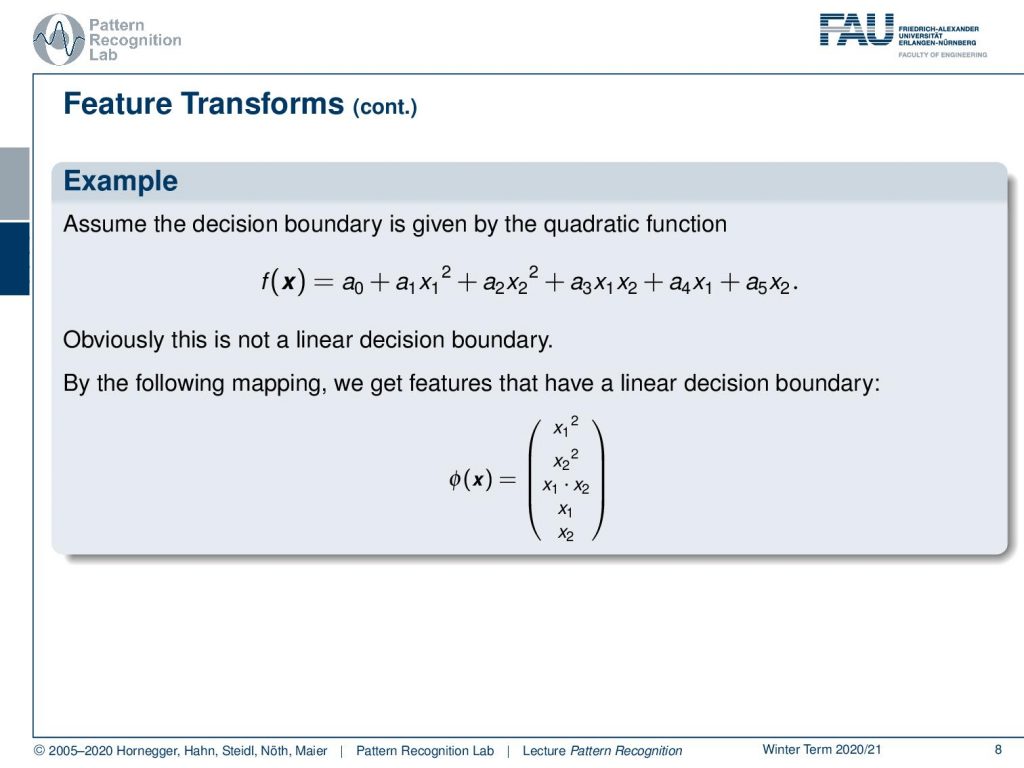
We’ve seen that the decision boundary given by quadratic functions is not linear. But because the parameters in a are linear, we can map this to this high-dimensional feature space to get linear decision boundaries in this transformed high-dimensional space.

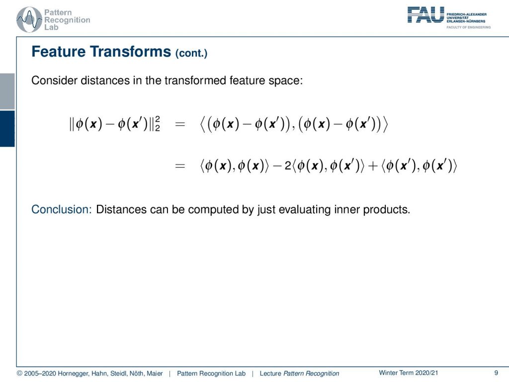
Now let’s consider the distances in the transform space. So I apply Φ, and I apply to some x and some x′ and take the L₂ norm. If we stretch this out, then you’ll see this is the inner product of the two differences. Then we can essentially write this up. And you’ll see that I get essentially only inner products. The L₂-Norm of our transform spaces can be written only by using inner products. So with this kind of feature transform, we can even evaluate distances only by the means of inner products. 

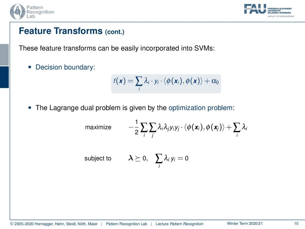
This then also means that they can very easily be incorporated into our support vector machine. So the decision boundary is then given as the feature transformed vectors using the inner product. Also, the optimization problem can be rewritten with this inner product, so we can integrate this quite easily also to the support vector machine.

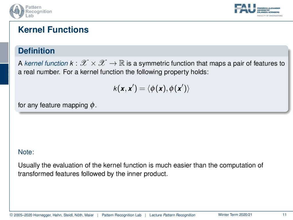
This then brings us to the notion of a kernel function. A kernel function that is mapping from two feature domains (that are both identical of course) x to some value R that is a real value. It needs to be a symmetric function that maps pairs of features to real numbers. And in this case, then the property holds that our k is given as the inner product of the feature transforms of the respective x and x′ for any mapping Φ. So this is usually much easier to evaluate because we only need to have the inner products. And if we have a finite set of training observations we can of course precompute those.

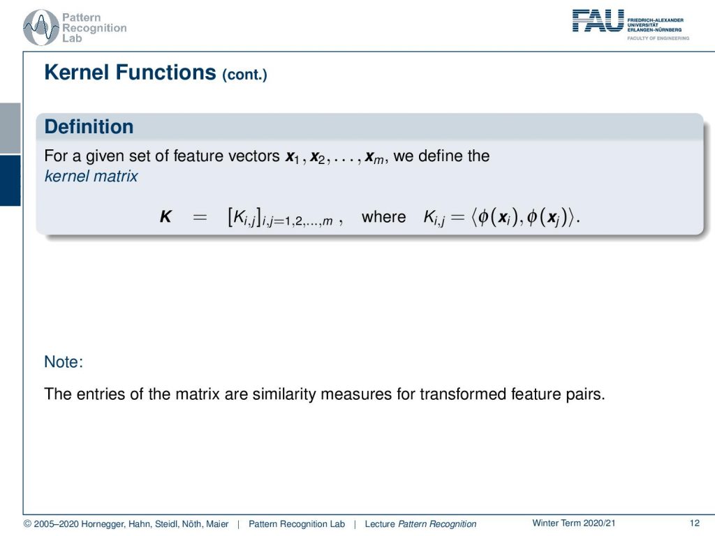
If you pre-compute those, this gives you the kernel matrix. In the kernel matrix then you have all the elements that are essentially the inner products of the feature transforms. So all of these entries are similarity measures of the transformed feature pairs. 

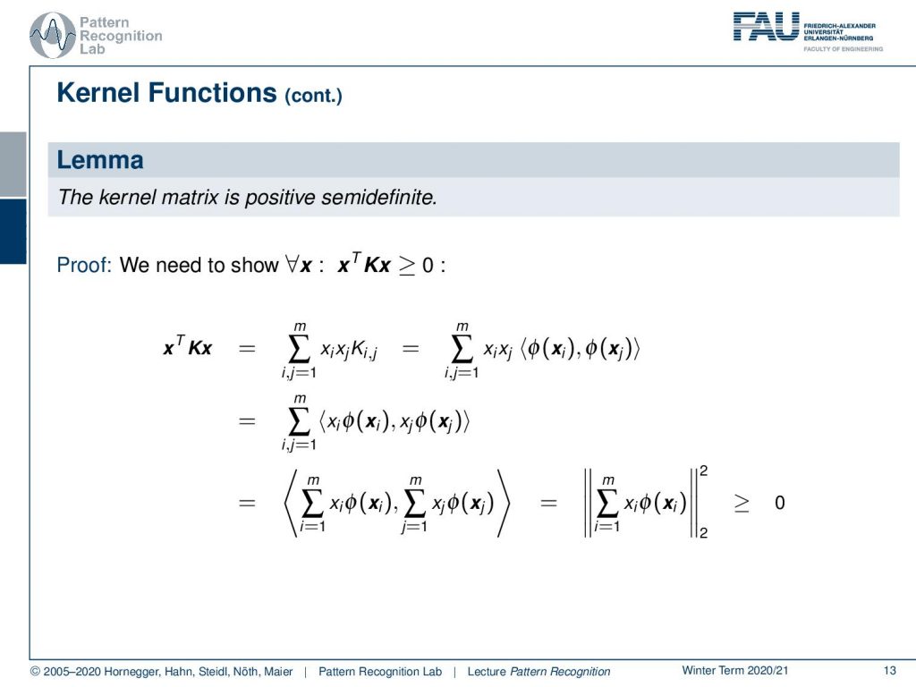
This kernel matrix is positive semidefinite and we can actually also show this. We know that the property needs to be fulfilled for all x, that x^TKx is greater or equal to zero. So let’s start with this. We can rearrange this and write it as a sum. So we see that these are the entries of K_i,j multiplied with x_i x_j. Then we see that the entry of K is simply the inner product of the feature transforms. This then means that we can bring in also the x_i and the x_j into this transform. You’ll see here that the sum is a linear operation, so I can also bring the sum into the respective inner product. Now you can see that this is an inner product of the respective sums. This is essentially two times the same sum, but with different indices. This then means that this can be rewritten as the average over x_i times Φ(x_i). This is an L₂-norm, and the L₂-norm is of course always greater or equal to zero. So we can easily show that this is positive semidefinite.

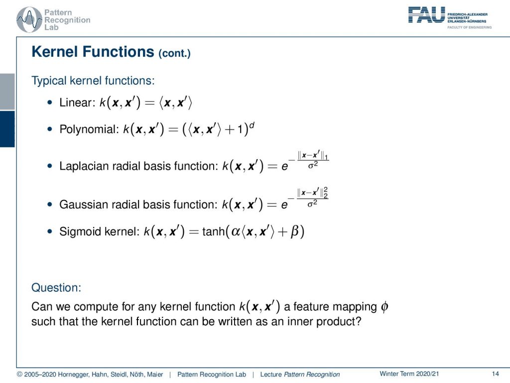
Let’s look into typical kernel functions. There is the linear kernel that you’ve already seen. We’ve talked about the polynomial one. A new one that I want to suggest here is the Laplacian radio basis function. There we are essentially using e to the power of minus, and then not the L₂-norm but the L₁-norm, and we divide by some standard deviation. Obviously, we can do something similar to Gaussians where we then have the L₂-norm. We can also use sigmoid kernels using the hyperbolic tangent. And now the real question is: can we find for every kernel function a feature mapping Φ such that the kernel function can be written as an inner product? This is an important question for us because only then do we have this property with the inner product that we use so heavily. 

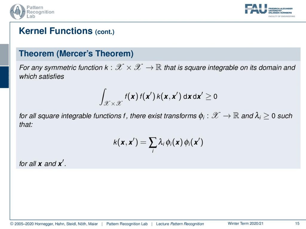
There is Mercer’s Theorem, and Mercer’s Theorem tells us that any symmetric function that maps a feature space let’s say x times x, so this is a function of two variables, to a real space and that is square-integrable on its domain and satisfies this integral here. The integral over the whole domain of f(x) f(x′) k(x,x′)dxdx′ is greater or equal to 0. For all square integrable functions f, there exists a Φ_i from 𝒳 to ℝ and λ_i greater 0 such that this kernel function k can be expressed as a sum over λ_i’s and feature transforms Φ_i(x)Φ_i(x′) for all x and all x′.

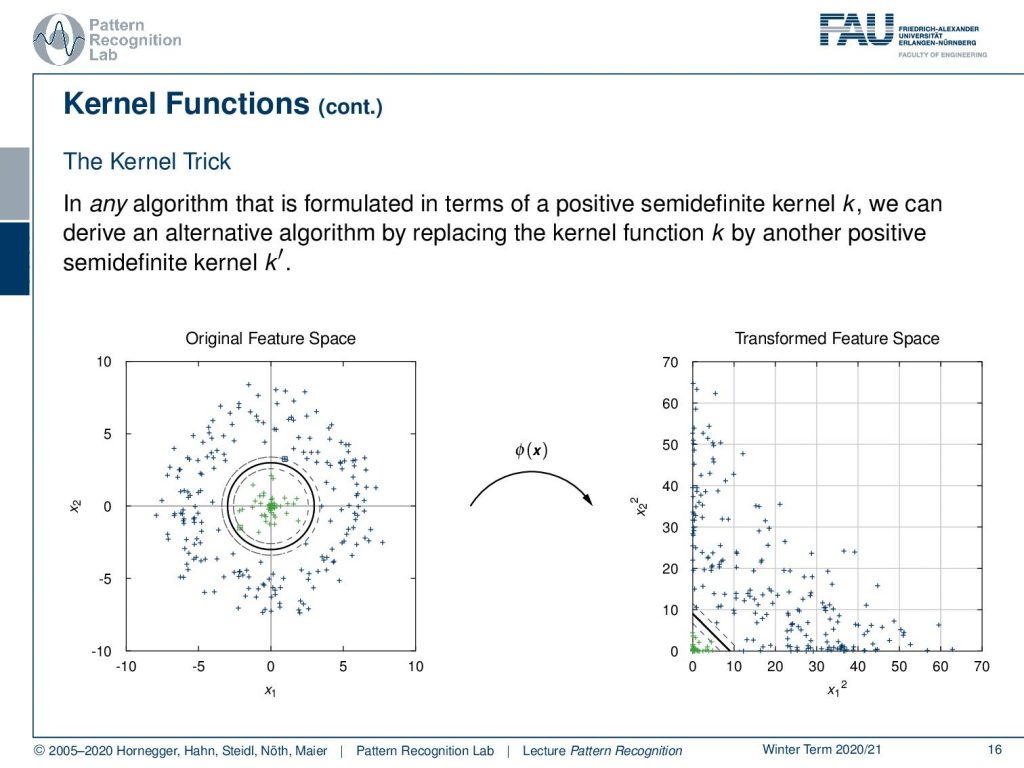
Now, this brings us to this Kernel trick. In any algorithm that is formulated in terms of a positive semidefinite kernel, we can derive an alternative algorithm by replacing the kernel function k by another positive semidefinite kernel k′. We see the original feature space and we apply our feature transform. And this is our transformed feature space, so the Kernel Trick. Now in this transformed features space, we have this very nice property of being linearly separable.

Let’s look back at our kernel SVM with soft margins now. This is the linear kernel here where the complexity parameter C controls the number of support vectors and hence the width of the margin and the orientation of the decision boundary. So we can see that here. If we vary C then you see that the number of support vectors is increased and so also our decision boundary changes. 

Now we can apply the same idea in polynomial space. And now if I project the polynomial decision boundaries and margins back into the original domain, you can see here how the decision boundary is displayed in the original data space. So you see here the polynomial kernel and the margins. Now if I decrease C you can see how the margin area is increased.

Of course we can also use other kernels like the gaussian radial basis function kernel here. and here you can see now that we get a decision boundary and our margins are essentially encircling the two classes here. So, very interesting. And of course, we can then also color code the output of our decision boundary. And you’ll see that at the zero level set the actual decision boundary is. And then also you’ll see that the one class here is then indicated in blue and the other class is indicated in red. So this was a short introduction to kernels and Mercer’s Theorem.

In the next video, we want to talk about further applications of kernels, and we want to introduce concepts like the kernel PCA. You remember we could also write this up as inner products, so this can also be applied to general feature transforms. And we also want to talk about a couple of additional advanced kernels. Thank you very much for listening and looking forward to seeing you in the next video! bye-bye. 

If you liked this post, you can find more essays here, more educational material on Machine Learning here, or have a look at our Deep Learning Lecture. I would also appreciate a follow on YouTube, Twitter, Facebook, or LinkedIn in case you want to be informed about more essays, videos, and research in the future. This article is released under the Creative Commons 4.0 Attribution License and can be reprinted and modified if referenced. If you are interested in generating transcripts from video lectures try AutoBlog.

References

1. Bernhard Schölkopf, Alexander J. Smola: Learning with Kernels, The MIT Press, Cambridge, 2003.

• Vladimir N. Vapnik: The Nature of Statistical Learning Theory, Information Science and Statistics, Springer, Heidelberg, 2000.

• John Shawe-Taylor, Nello Cristianini: Kernel Methods for Pattern Analysis, Cambridge University Press, Cambridge, 2004

Category: Lecture Notes in Pattern Recognition