Lecture Notes in Pattern Recognition: Episode 25 – Support Vector Machines – Optimization

These are the lecture notes for FAU’s YouTube Lecture “Pattern Recognition“. This is a full transcript of the lecture video & matching slides. We hope, you enjoy this as much as the videos. Of course, this transcript was created with deep learning techniques largely automatically and only minor manual modifications were performed. Try it yourself! If you spot mistakes, please let us know!

Welcome back to pattern recognition. Today we want to talk about support vector machines. But we want to remember what we learned about duality and convex optimization and applied it to our support vector machines here. So, let’s see what we can learn more about support vector machines.

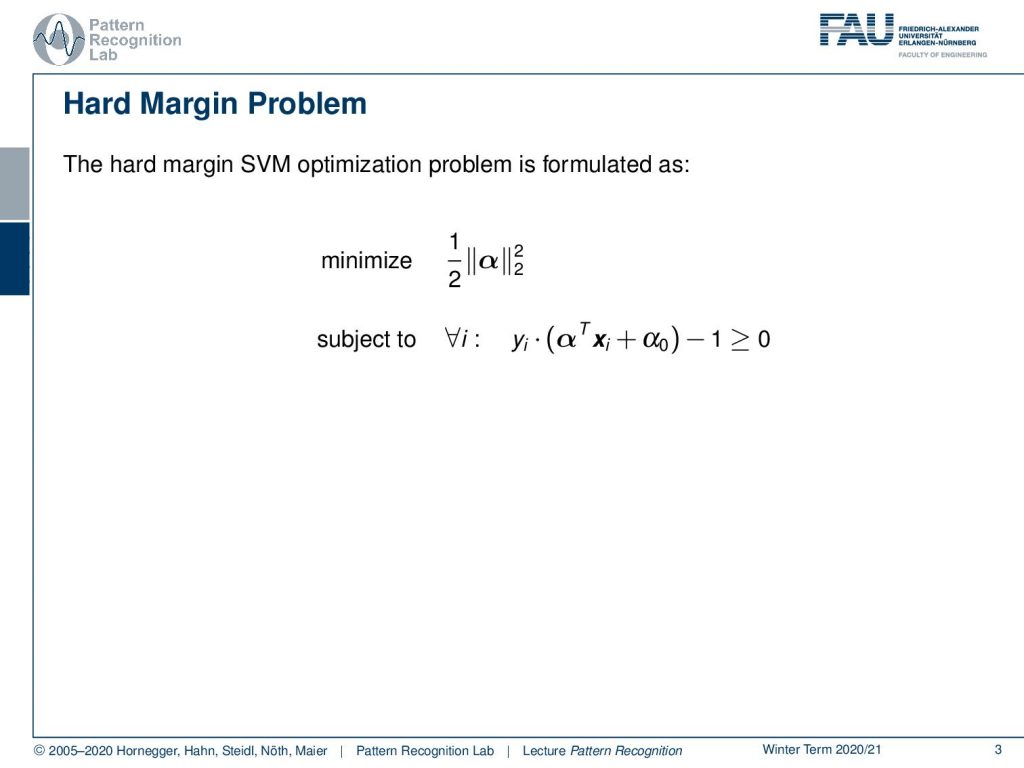
This is the second part of support vector machines and we’re back to the hard margin problem. Here we see that the SVM can be formulated as the norm squared of our α vector. You remember α is essentially the normal vector of our decision boundary. Then we have to constrains our y_i that is multiplied essentially with the signed distance to the decision boundary. This -1 needs to be larger or equal to zero because we want to preserve this margin. 

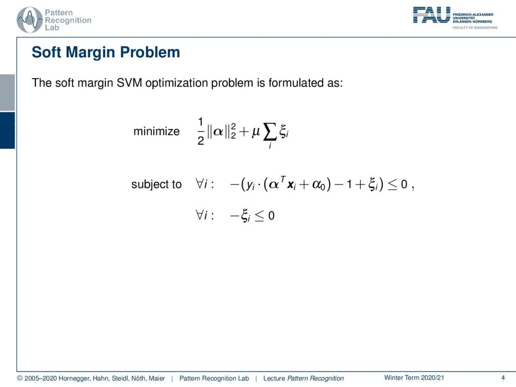
In the soft margin case, you remember that we introduced additional slack variables. So here we had the ξ_i and the ξ_i should help us to move points that were on the wrong side of the decision boundary back to the correct side. We will then also be able to find solutions in cases where the classes are not linearly separable. We also need to adjust our constraints to include x_i and we also need to put in an additional constraint with the – ξ_i being smaller or equal to 0. 

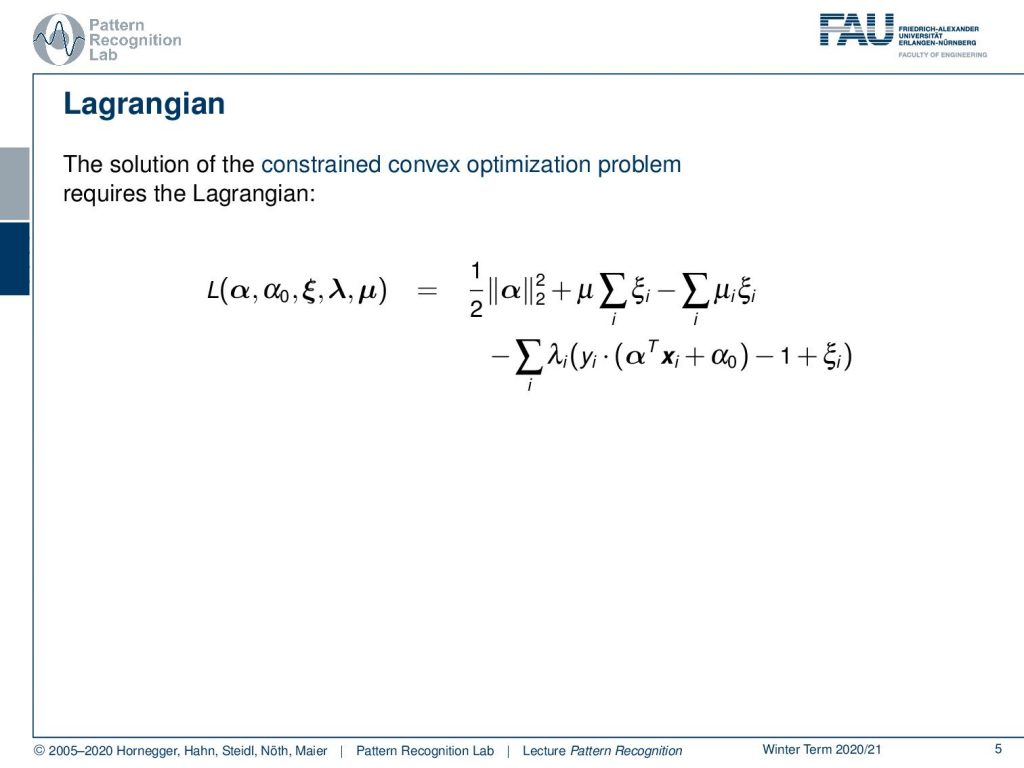
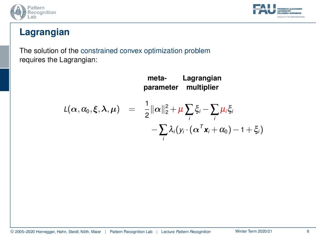
Now let’s set this up in the Lagrangian. So the solution of the constrained convex optimization problem requires this Lagrangian function. So here you have the norm of the normal vector to the power of 2 and then you have some μ times the sum of over ξ_i. Then, we have the minus sum of μ_i ξ_i and we have the minus sum over our constraints and this is then employing λ. 

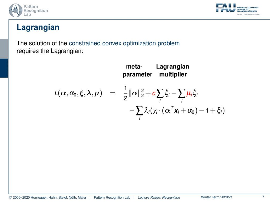
So one thing that we can do is this: μ, we can essentially map this into a meta parameter and therefore we then can essentially remove this from the optimization because we choose this as a constant c. 

We see that we have the Lagrangian multipliers the μ_i and the λ_i. 

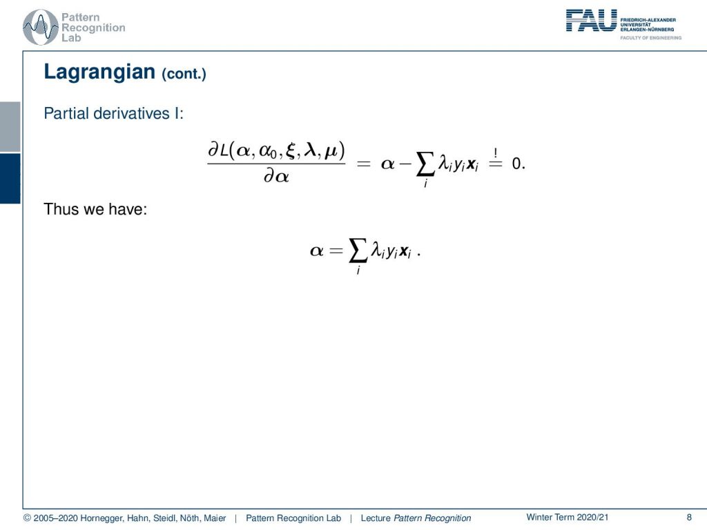
Now, if we go ahead and then compute the partial derivatives of our problem here with respect to our parameter α you see that this is going to give you α minus the sum of λ_iy_ix_i and this needs to be zero. So we can solve this and this gives us α as the sum of λ_iy_ix_i and this somehow seems familiar, right? We’ve seen similar update rules already in the case of the perceptron where we had this y_i multiply with x_i as an update step. Here, we see now if you have to sum over the entire training dataset, we can essentially map this to our original parameter α. So that’s a very interesting observation. We can express the variable that we are actually looking for under primal problem completely by the training dataset and our Lagrange multipliers. 

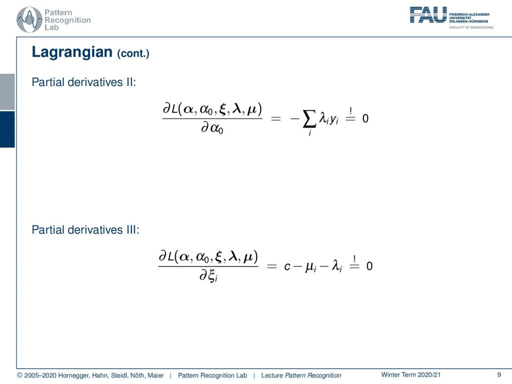
Let’s look at some more partial derivatives. The partial derivative of the lagrangian with respect to α₀ is simply going to get minus the sum over λ_iy_i needs to be zero. The next partial derivative is going to be the one with respect to ξ_i and this is gonna give c-μ_i– λ_i and this is required to be 0. 

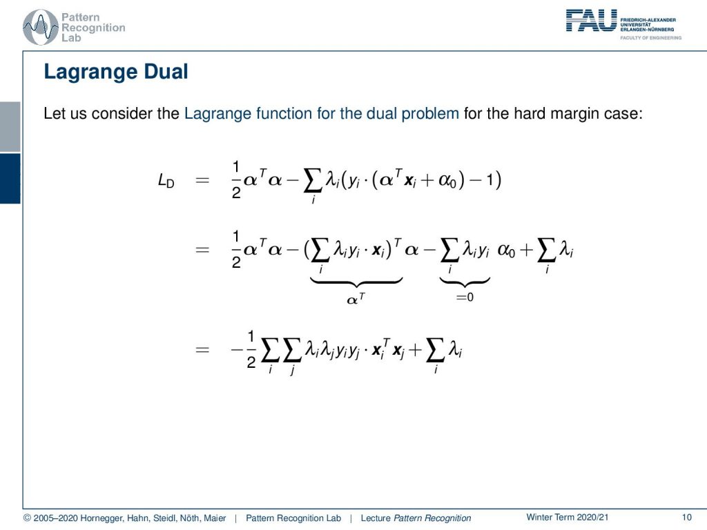
So if we now use this in our Lagrangian function, we can see here this is the Lagrangian function for the hard margin case. Then we can rearrange this a little bit so you see that I can put out the α from the sum and rearrange the sums a little bit and here then see that we essentially get for the second term and the sum that it contains the λ_iy_ix_i transpose. So this can be replaced with α transpose. Then the third element here is the sum of the λ_iy_i this needs to be 0. Then we see that we still have to sum over the λ_i. So we can now essentially write this up as a sum over the λ_iλ_jy_iy_ix_i^Tx_j plus the sum over the λ_i. So this is also interesting, because now in the dual, we don’t have the original α anymore. So α was actually the variable that we were optimizing for in the primal and here you see that this allows us to rearrange the dual and in the dual we do not have the α anymore. So we don’t even have to work with this infimum and so on as we have seen earlier. We’re able to derive the Lagrange dual function directly from the primal optimization problem. So this is a very interesting observation. Also, note that our problem is strictly convex. So we can find a very nice solution here for the dual. 

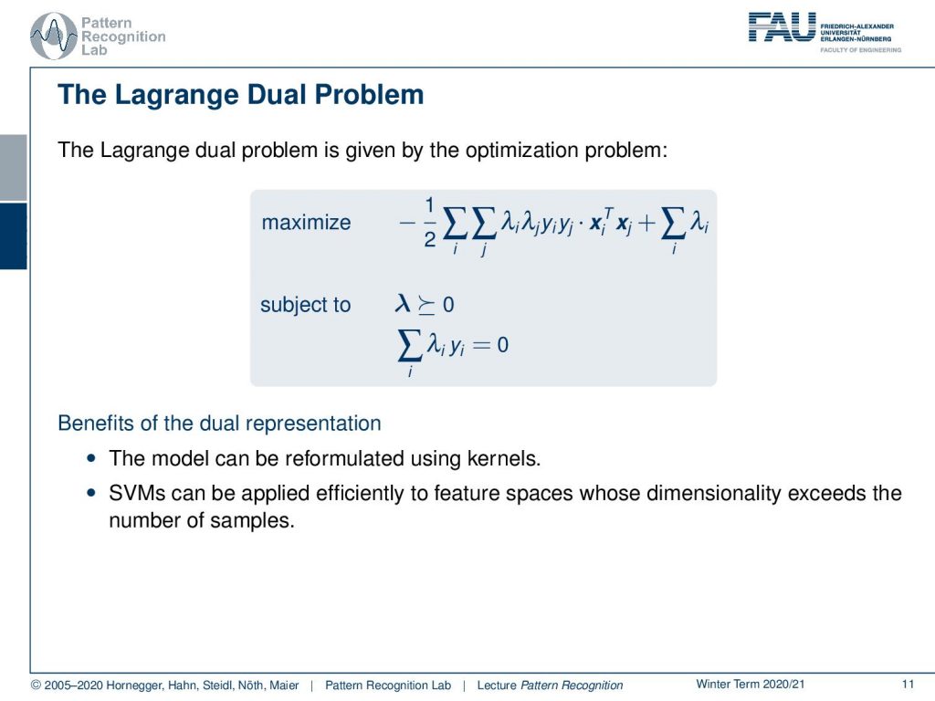
So this is then leading us to the following optimization problem. The Lagrange dual problem where maximize – 1/2 and then this double sum of the λs, ys and Transpose of x size plus the sum of the λs subject to that all the λs are greater than 0. Of course, we still have to put in the constraint that the sum of multiplication of the λ_i and y_i need to be one. So this still has to be fulfilled although it fell out of the primal equation. This has a couple of benefits that we can see now. So this model can be reformulated using something that is called a kernel because our training dataset only appears in terms of inner products. So we essentially only need to compute the x_i^Tx_j and this is an inner product of the two feature vectors. This is also very interesting because of the actual dimensionality of the feature space, we don’t care because we just have this in a product. So we can apply this very efficiently in high-dimensional spaces because it doesn’t change our complexity that much. Essentially if we’re able to precompute all those inner products then we wouldn’t change the complexity of the training process at all. Because we are able to optimize in this inner kernel inner product space. So this is actually a pretty cool observation.

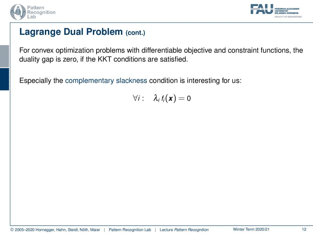
So for convex optimization problems with differentiable objective and constraint functions, we know that the duality gap is zero if the KKT conditions are satisfied. This then allows us also to work with the concept of complementary slackness. This is particularly interesting for us. 

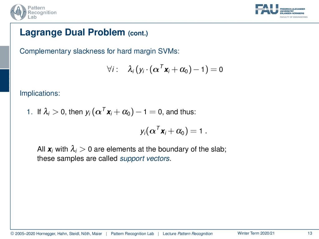
You remember this is λ_i times the bracket is equal to 0 for all i and if we now apply this to our hard margin SVM, then you can see that we can rearrange this here a little bit. It essentially means if we have a λ_i that is greater than 0 then the y_i(α^Tx_i + α₀) is zero. So this means that the respective observation of x_i lies exactly on the margin line. So these are essentially the two lines that are 1 away from the decision boundary. We have the margin lines on both sides of the decision boundary but all the points that have a non-zero λ are points that lie exactly on the decision boundary. Now, this brings us to the notion of support vectors as so you have to understand the Lagrange dual problem, complementary slackness, and everything if you want to explain what support vectors are. Because support vectors are all the observations in the training dataset where we then find Lagrangian multipliers that are greater than zero. So this is a very interesting observation and if you have a question like what is this support-vector in the support vector machine, it sounds like a very easy question but actually, you need to explain all those concepts in order to explain this to somebody what the notion offer support vector actually is. Now, this is actually cool because we’ve seen that the normal of our decision boundary can be expressed as the sum of the product of λ_iy_ix_i. Now we know that λ_i is going to be 0 for all of the observations that are not part of the margin lines of our decision boundary. So this means that essentially at the end of our training process, we have some observations of the λs and the λs essentially tell us which factors we actually need to store in order to describe the decision boundary correctly. So that’s also really cool because it intrinsically selects only the relevant vectors from our training dataset and with these relevant factors we can then construct the decision boundary. So that’s also a super cool observation. 

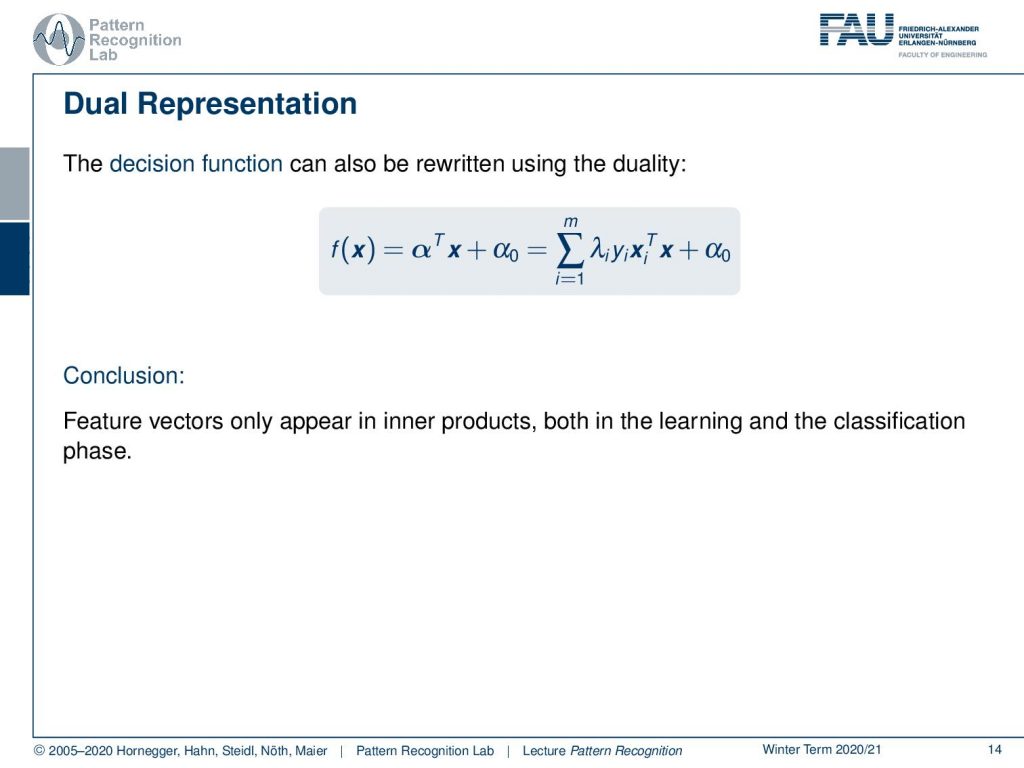
So let’s go back to our dual representation. We now see that this decision boundary can be rewritten only as of the actual use of the support vectors. So they have the sum over λ_iy_ix_i transpose the new observation x plus some α_0. So if you know the support vectors and α₀, then we can actually determine the decision boundary using only our support practice. This is also really cool and you’ll see that our feature vectors only appear as inner products in the learning and in the classification phase. So you see that we intrinsically can work with very high dimensional spaces and this then brings us back to feature transforms where’s the right now only able to describe linear decision boundaries. 

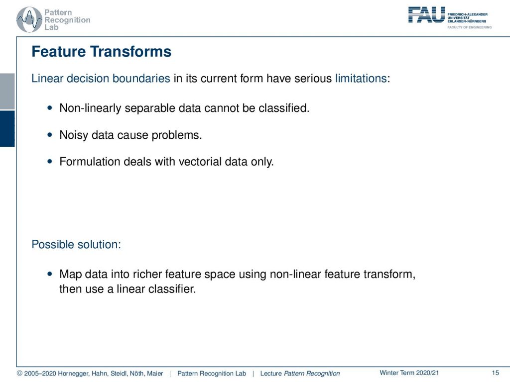
This, of course, has serious limitations because if we have non-linearly separable data it can be classified or we can work with the slack variable of course. Then we can, of course, find a solution but it will still only be linear and it might not be a very good solution. We will see a couple of examples and also noisy data can cause problems. So this formulation is dealing with vectorial data only right now. Now, we have seen already the idea that we can map our data into a higher-dimensional space and this is done using a non-linear feature transform. Then we use a linear classifier. 

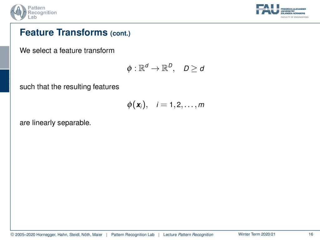
So we use a feature transform where we now go with a fine from a dimensionality of d to D and D is actually a much higher dimensionality. Now, are we then have essentially resulting features that are generated with the feature transform ϕ(xi) and this is of course done for our entire training dataset. The resulting features will then be linearly separable. 

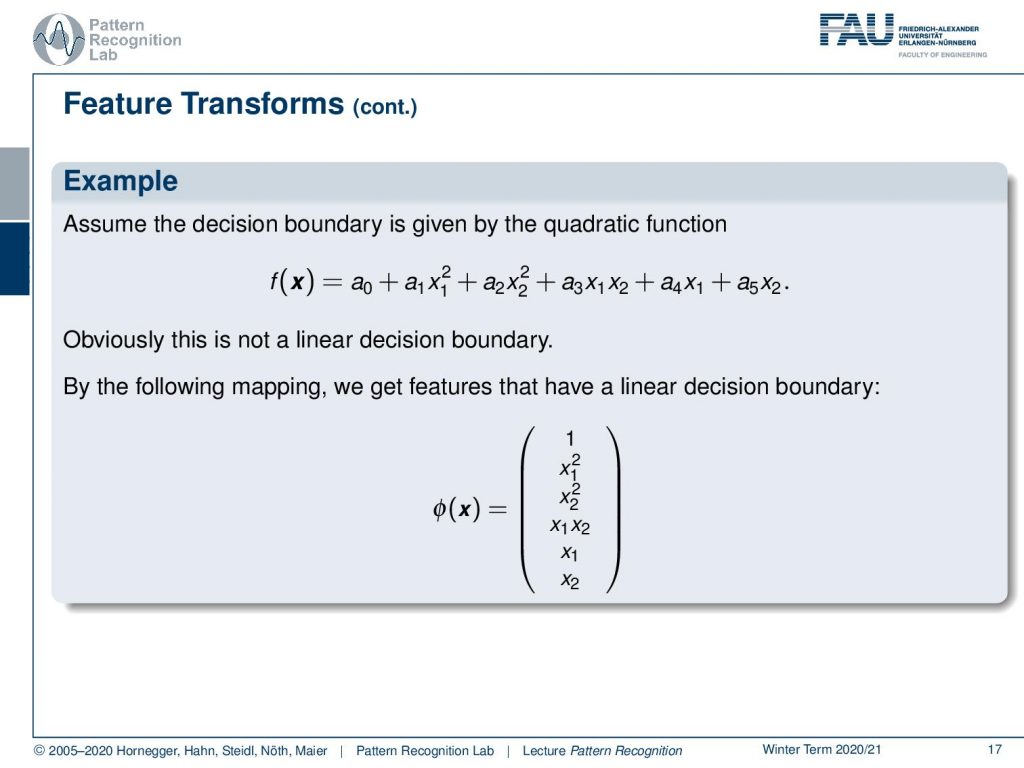
So let’s look into one example let’s assume that the decision boundary is given by this quadratic function. Then it’s quite obvious that this is not a linear decision boundary. But we can rearrange this function and then we have suddenly a linear decision boundary because if you use this ϕ(x). Then we can essentially see that our polynomial is linear in the coefficients. If he had applied this mapping then we just have an inner product of our vector a and the ϕ(x). So suddenly we have a  linear decision boundary in this high-dimensional space.

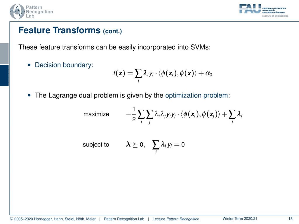
Now you see that this then alters our SVMs. In the end, we have the decision boundary that is now given as the sum of a the λ_iy_ix_i and now this inner product using this feature transformed plus α₀. So the Lagrange dual problem is that given by the following optimization problems. So we maximize our double sum over λ_iλ_jy_iy_j and the inner product of the two feature transformed feature vectors plus the sum of all the λ_i and again we have these additional constrained as we’ve seen previously. This is interesting because this essentially allows us to define something that we call a kernel function.

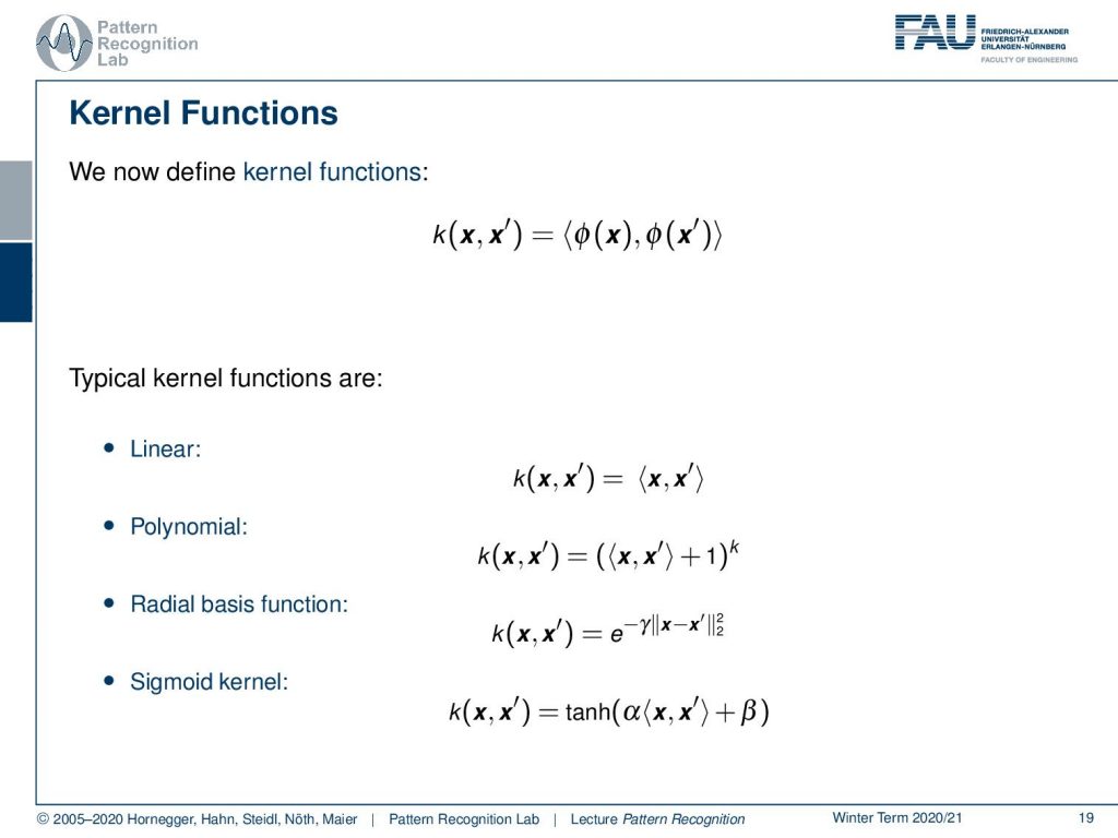
Now if you have a kernel function that is k of x and x’ then we have essentially the inner product of ϕ(x) and ϕ(x’). We see that with this trick of the kernel we can essentially construct a lot of different functions that follow this idea. We’ve already seen the linear one and it recently had into the relation. We’ve seen the trick with the polynomial that you can then construct this by an inner product of x and x’ plus 1 to the power ok k which defines the degree of the kernel. You can use the Radial basis function. So there you essentially take the two Norm of the difference of the two vectors and then plug into something that is e to the power of –γ. You can also work with sigmoid kernels where you can use for example this hyperbolic tangent here. So all of these kernels are feasible and they can be used and essentially be precomputed. We will look into a couple of examples in the next video, we then want to talk about kernels. 

What you learned here is that the Lagrangian formulation can be done with hard and soft margin problems. We looked into the Lagrange dual formulation and we introduce this idea of feature transforms which we will discuss in much more depth in the next video where we don’t talk about kernels again.

I have some further readings for you. Bernhard Schölkopf and Alex Smola’s Learning with Kernels, Vapniks’s Fundamental Publication Again by then Vandenberghe Convex Optimization and also the book by Bishop Pattern Recognition and Machine Learning.

Again, I prepared some comprehensive questions for you. So, this then already brings us to the end of this video. I hope you liked the small overview of support vector machines and how convex optimization can help us in finding the dual problem and with the dual problem with and found very interesting properties of the primal problem including the notion of the support vectors. So, thank you very much for listening and looking forward to seeing you and the next video. Bye-bye!! 

If you liked this post, you can find more essays here, more educational material on Machine Learning here, or have a look at our Deep Learning Lecture. I would also appreciate a follow on YouTube, Twitter, Facebook, or LinkedIn in case you want to be informed about more essays, videos, and research in the future. This article is released under the Creative Commons 4.0 Attribution License and can be reprinted and modified if referenced. If you are interested in generating transcripts from video lectures try AutoBlog

References

1. Bernhard Schölkopf, Alexander J. Smola: Learning with Kernels, The MIT Press, Cambridge, 2003. 
2. Vladimir N. Vapnik: The Nature of Statistical Learning Theory, Information Science and Statistics, Springer, Heidelberg, 2000. 
3. S. Boyd, L. Vandenberghe: Convex Optimization, Cambridge University Press, 2004. ☞http://www.stanford.edu/~boyd/cvxbook/ 
4. Christopher M. Bishop: Pattern Recognition and Machine Learning, Springer, New York, 2006

Category: Lecture Notes in Pattern Recognition