Lecture Notes in Pattern Recognition: Episode 24 – Duality in Optimization

These are the lecture notes for FAU’s YouTube Lecture “Pattern Recognition“. This is a full transcript of the lecture video & matching slides. We hope, you enjoy this as much as the videos. Of course, this transcript was created with deep learning techniques largely automatically and only minor manual modifications were performed. Try it yourself! If you spot mistakes, please let us know!
Welcome back to Pattern Recognition! Today we want to look a bit more into convex optimization. In particular, I want to introduce you to the concept of duality in convex problems.
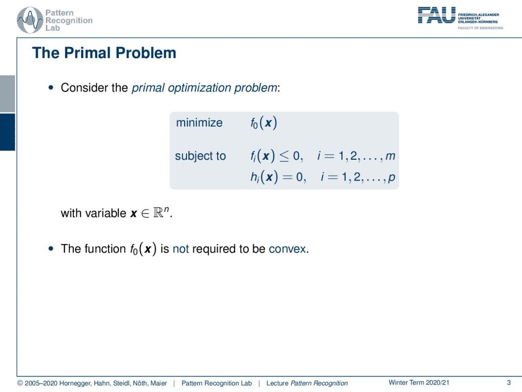
Let’s have a look at duality in convex optimization. If we want to look into something dual we have to differentiate essentially two problems, there is the primal problem and the dual problem. So let’s start with the primal problem. This is an optimization problem as we’ve seen them before. We want to minimize some function f0(x), and this is subject to some constraints. Here we have two sets of constraints, there are the fi(x), which are inequality constraints, and then we have the hi(x) which are equality constraints. Note that this doesn’t necessarily have to be convex functions. So duality is generally a concept that you can introduce whenever you’re dealing with constrained optimization. Let’s look into the Lagrangian that emerges then from this one here.
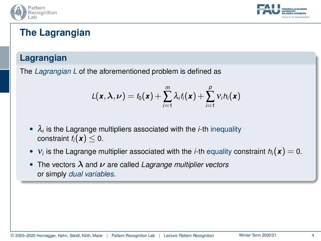
Of course, we can build the Lagrangian function. This is one, and this is the primal f0 plus then the inequality constraints multiplied with λi and summed up and then the equality constraints multiplied with νi and summed up. Again we use the trick that we move from an n-dimensional space to a space of higher dimension. Here we increase the dimensionality by m, the number of inequality constraints plus p, the number of equality constraints. We’ve seen that these are the Lagrange multipliers, this is the inequality one this is the equality one. Now we have a set of new vectors that are λ and ν and these are our Lagrange multipliers. They are also called the dual variables, so this is the step towards the dual problem.
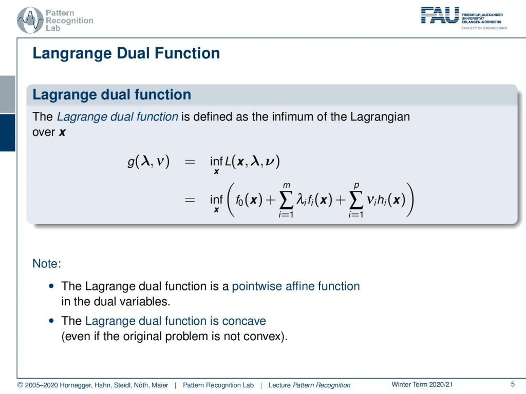
Now let’s look into the Lagrange dual function. In the Lagrange dual function now we essentially get rid of x. Essentially we want to pick x in a way such that we get the maximum lower bound of our lagrangian function. So we can write this up as g(λ, ν) is the infimum over x of our lagrangian function. And we can essentially expand this here. This is of course then the infimum over f0(x) plus the inequality constraints plus the equality constraints. This is interesting. You can note here already that the Lagrange dual function is a pointwise affine function in the dual variables. Also, the Lagrange dual function is concave. So the introduction of this infimum makes our function concave even if the original problem is not convex.
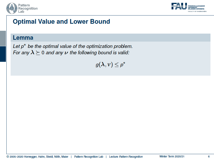
Now let’s introduce some p* that is the optimal value of the optimization problem. Then for any λ greater to zero and any ν the following bound is valid. The p* is an upper bound for our Lagrange dual. So this is the maximum value that can be attained by the Lagrange dual function. Let’s look at some examples!
Let’s start with our primary function f0(x) that we see here. Now we introduce the first constraint. This is f1(x). Now let’s align them here so that you can see where the same points are. And now we can start building the Lagrange dual function. And of course, we have to introduce some kind of λ to mix the two.
We start with a λ of 0.1. Now we are interested in the largest value of x that is a lower bound for this function. So you can see now when I start increasing the value of λ, that we are deforming the original function. And you can see actually in about this position here we have some upper bound that is higher than the previous upper bounds. Because we got rid of the negative lobe on the left-hand side and also in the center we kind of have a very high upper bound that we can choose here. Now if I start increasing λ more, you see that the center lobe goes down and our maximum lower bound is already going down again. So you can see that we essentially can write this up as a function of λ.
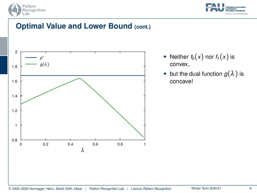
If we now plot this differently, you can see that there is our p*, which is just a fixed value. This is the optimal value of our optimization problem. And you can see if we vary λ, then the value of our Lagrange dual, this infimum, is slowly increasing up to some point we are already pretty close to p* and then it is decreasing again. So in our example neither f0(x) nor f1(x) is convex but the dual function is concave. This is a very interesting observation. Now let’s look into this a little bit more.
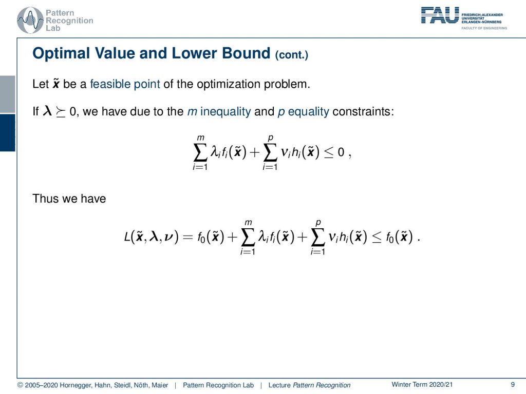
We can see that if we have a feasible point of the optimization problem. This is x̃, a point that essentially fulfills the constraints. And we have our λ greater or equal to zero. Then, because of the m inequality and p equality constraints, we can essentially see that the sum over our lagrangian multipliers has to be lower than zero. Because, if the equality constraints are fulfilled, of course, the right-hand term is zero and the left-hand term is negative because it is an inequality constraint. So this term, this double sum here, is always lower than 0 for any feasible point, meaning points that fulfill the set of constraints. This means that if we have a feasible point in the Lagrange function, then we can see that at a point x̃ we have an upper bound for the Lagrange function that is f0(x̃). This is also a very interesting observation that if we have points that fulfill the constraints, then we essentially know that there is an upper bound of the original optimization problem f0.
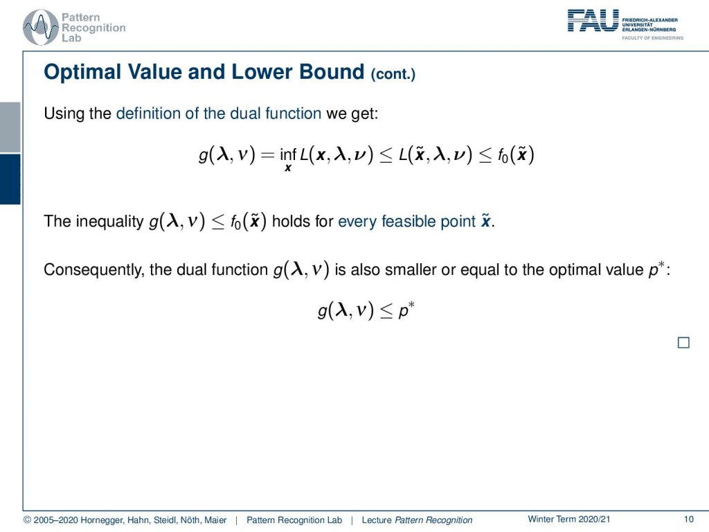
Now we can also use the definition of the dual function. Here we can see now that if we have g(λ, ν) this is essentially the infimum over our Lagrange function. This is bounded as an upper bound by the position x̃ and same function. We can see there is an even higher bound that is f0(x̃). This inequality that f0(x̃) is greater or equal to the Lagrange dual function holds for every feasible point x̃. This also then means that if we have an optimum value, this optimal value needs to be larger than the actual Lagrange dual function.
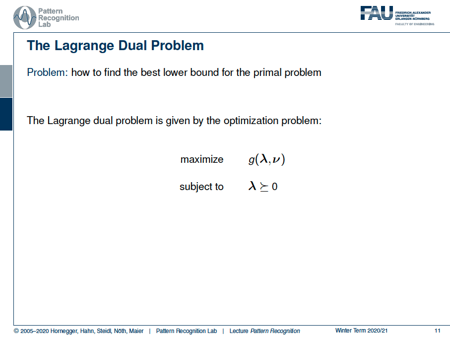
This then brings us to the problem of how to find the best lower bound for the primal problem. This can then be done by maximizing the Lagrange dual function. At the same time, we want our λ to be greater or equal to 0 because these are the Lagrange multipliers that are associated with the inequality constraints. Now let’s look into something that is called the duality gap.
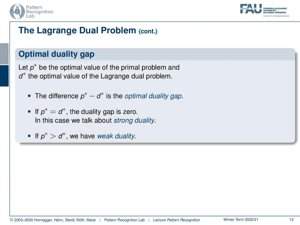
So let p* be the optimal value of the primal problem, and d* the optimal value of the Lagrange dual problem. Then we can define a difference between p* and d*, and this is called the optimal duality gap. If p* equals d*, then the duality gap is zero. In this case, we have a condition that is called strong duality. In cases where we can’t attain this, where our p* is greater than d*, then we have weak duality. Now let’s look into something that is called Slater’s Condition.
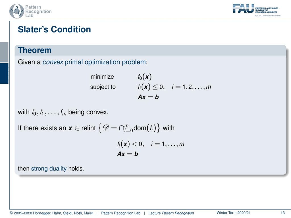
There’s this nice theorem. This tells us if we have a convex primal optimization problem where we have some f0 and fi and then some equality constraints and all of the inequalities and also f0 is convex. Then, if there exists an x that is an element of the relative interior that we can here essentially define as the intersection of all of the domains of the fi, and in this constraint the inequality constraints and the equality constraints hold, then we have strong duality. There’s also a different version of this. If the first k constraints are affine and there exists an x in the relative interior with the affine inequality and the convex inequality constraints as well as the equality constraints fulfilled, then strong duality holds.
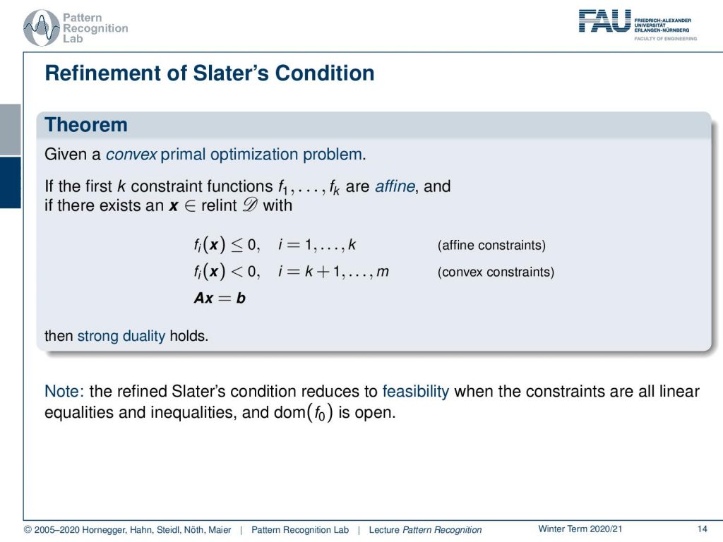
Now, this refined status condition essentially reduces to feasibility when the constraints are all linear equalities and inequalities and the domain of f0 is open. In these cases, we simply require the feasibility of x.
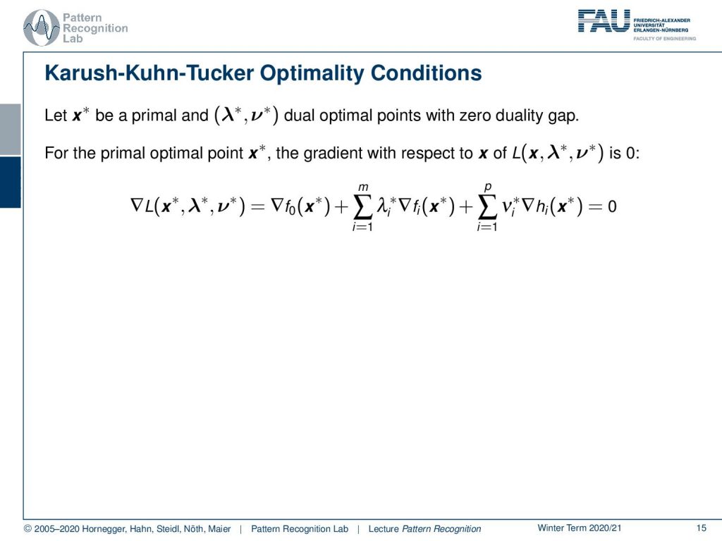
This then brings us to the Karush-Kuhn-Tucker optimality conditions. Let’s find the optimal points of the primal and dual problems. Here x* is going to be the optimal solution for the primal, and λ* and ν* are the optimal points of the dual problem. If there is a zero duality gap then we can use the Karush-Kuhn-Tucker optimality conditions. They are essentially related to the condition that the gradient for x of the Lagrangian is zero. If we compute this gradient, then we can spell this out as the gradient of f0(x) at x* plus the gradient of the inequalities, plus the gradient of the equality constraints, and this equals zero.
Now there are four KKT conditions. They are related to the optimization problem. They include the primal constraints, meaning that the constraints of course have to be fulfilled. All of the inequality and the equality constraints have to be fulfilled and the dual constraints. This means that our λ’s need to be greater than zero. Then there is something that is called complementary slackness. There is this constraint that λi times fi (x) equals 0. This is a very interesting observation because it means that either the Lagrange multiplier is zero or the constraint is zero. So either of the two cases. Then we have zero, and we will see how we can find this complementary slackness in the next couple of slides. This is a very important concept that we’ll use in the support vector machine quite frequently. Then also the gradient of the Lagrangian is zero. These are the four KKT conditions, the primal constraints, the tool constraints, complementary slackness, and the gradient of the current gene is zero. So if strong duality holds and if x*, λ* and ν* are the optimal points, then the KKT conditions hold.
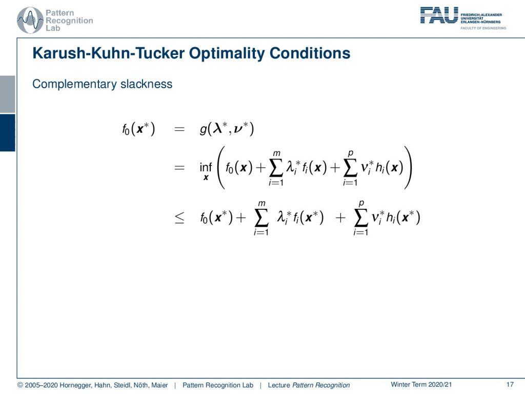
Let’s look into this concept of complementary slackness. This sounds a bit crazy, but we can derive this very quickly. Let’s start with f0(x*). Then we can see because of the strong duality this needs to be the same as the dual of λ* and ν*. Then we can plug in the definition. This is the infimum over our Lagrange function. Then we can see that this has an upper bound. The upper bound here is given of course, if we evaluate the Lagrangian at the position of optimality of the primal problem. So we plug in essentially x* here. This is an upper bound.
Now we can see that for this term here at the solution the constraint will be fulfilled. So this needs to be zero. And the inequality will also be fulfilled, so this needs to be lower than zero. And this means that we can find an upper bound for this. And this is simply f0 at x*. Now you realize that f0(x*) is popping up on both sides of our inequality. This means there must be an identity. Now, this also needs to be identical. So this is also not just an upper bound but also identical. And this then means that this term here is not a lower or equal, but also an equality. This means that this term here actually has to be zero. This is a sum over essentially positive constraints. This then means that the individual elements of the sum need to be 0. And this is exactly the complementary slackness.
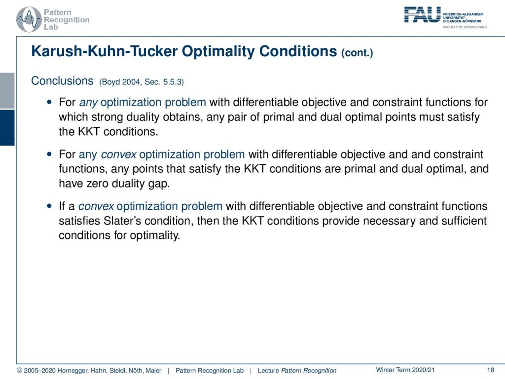
Let’s look at some conclusions here on the KKT conditions. For any optimization problem with differentiable objective and constraint functions for which strong duality obtains, any pair of primal and dual points must satisfy the KKT conditions. For any convex optimization problem with a differentiable objective and constraint functions, any points that satisfy the KKT conditions are primal and dual optimal and have zero duality gap. If a convex optimization problem with a differentiable objective and constrained function satisfies slater’s condition, then the KKT conditions provide necessary and sufficient conditions for optimality. We’ll see that slater’s conditions are important for the support vector machines. Therefore also the KKT conditions will apply in our support vector machines. This means that we can apply the concept of strong duality and look into the constraint optimization problem a little bit more.
What did we learn here? We found a way of formalizing the primal problem using the Lagrangian, we introduced the Lagrange dual function that is essentially getting rid of x at all using this idea of the infimum. Then we were looking into the duality gap, and we realized that in cases where there is no duality gap, we have the KKT conditions and also the concept of complementary slackness.

You see that we will apply the KKT conditions in the next couple of videos to the support vector machines. So this is what we will talk about in the very next video. We will immediately apply our new observations to the support vector machines and let’s see what comes out of that.
I do have some further readings for you. Again, “Convex Optimization” by Boyd and Vandenberghe. And, also a good read, “Numerical Optimization” here. I also prepared some comprehensive questions and I hope they help you with the preparation for the exam.
Thank you very much for listening and I’m looking forward to seeing you in the next video! bye-bye.
If you liked this post, you can find more essays here, more educational material on Machine Learning here, or have a look at our Deep Learning Lecture. I would also appreciate a follow on YouTube, Twitter, Facebook, or LinkedIn in case you want to be informed about more essays, videos, and research in the future. This article is released under the Creative Commons 4.0 Attribution License and can be reprinted and modified if referenced. If you are interested in generating transcripts from video lectures try AutoBlog.
References
- S. Boyd, L. Vandenberghe: Convex Optimization, Cambridge University Press, 2004. http://www.stanford.edu/~boyd/cvxxbook/
- Jorge Nocedal, Stephen Wright: Numerical Optimization, Springer, New York, 1999