Classical Activations
These are the lecture notes for FAU’s YouTube Lecture “Deep Learning“. This is a full transcript of the lecture video & matching slides. We hope, you enjoy this as much as the videos. Of course, this transcript was created with deep learning techniques largely automatically and only minor manual modifications were performed. If you spot mistakes, please let us know!
Welcome back to deep learning! So in today’s lecture, we want to talk about activations and convolutional neural networks. We’ve split this up into several parts and the first one will be about classical activation functions. Later, we will talk about convolutional neural networks, pooling, and the like.
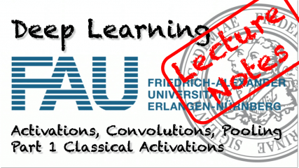
So, let’s start with activation functions and you can see that the activation functions go back to a biological motivation. We remember that everything we’ve been doing so far, we somehow also motivated with the biological realization. We see that the biological neurons are being connected with synapses to other neurons. This way, they can actually communicate with each other. The synapses have this myelin sheath and with this, they can actually electrically be insulated. They are able to communicate with other cells.
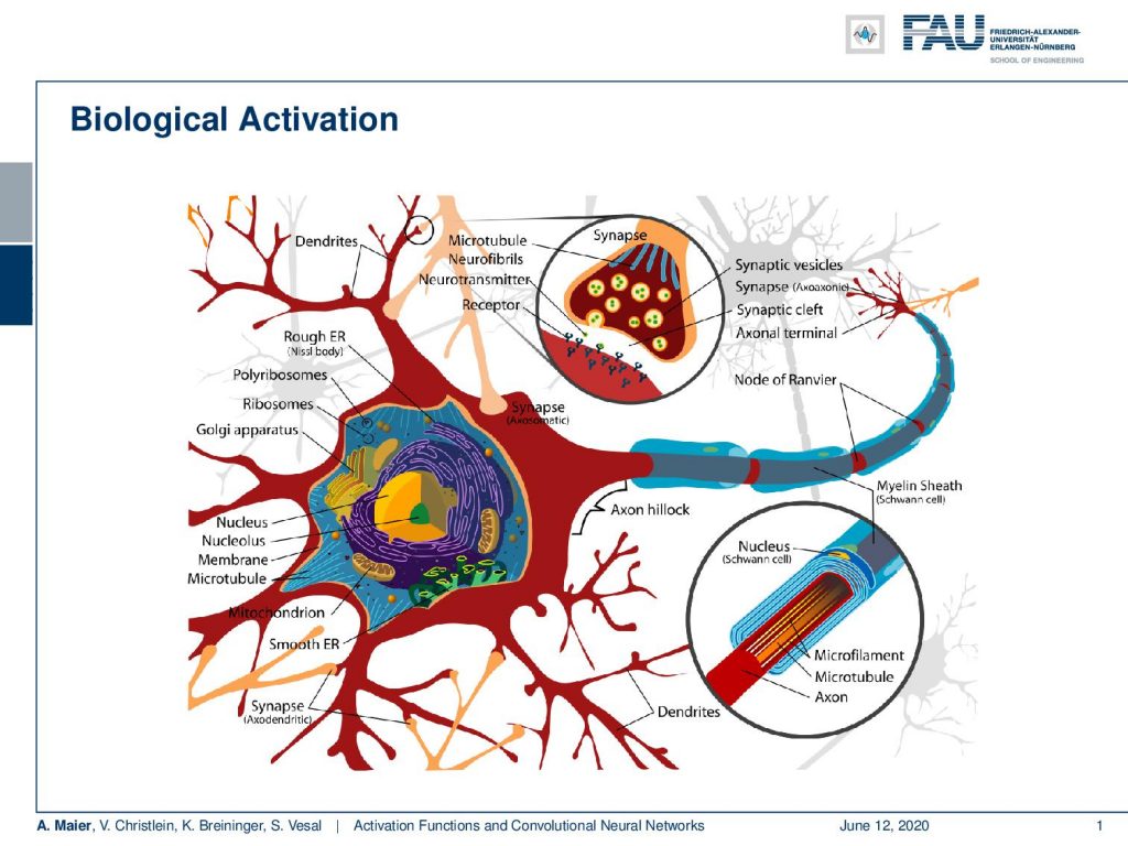
When they are communicating, they are not just sending everything that they get in. They have a selective mechanism. So if you have a stimulus, it actually does not suffice to generate an output signal. The total signal must be above a threshold and what then happens is that an action potential is triggered. After that, it repolarizes and then returns to the resting state. Interestingly, it doesn’t matter how strongly the cell is activated. It is always returning the same action potential and returns to its resting state.
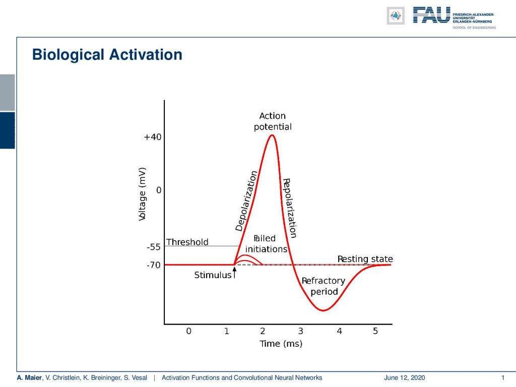
The actual biological activation is even more complicated. You have different axons and they are connected to the synapses in other neurons. On the paths, they are covered within Schwann cells that then can deliver this action potential towards the next synapse. There are ion channels and they are actually used to stabilize the entire electrical process and bring the whole thing again into equilibrium after the activation pulse.
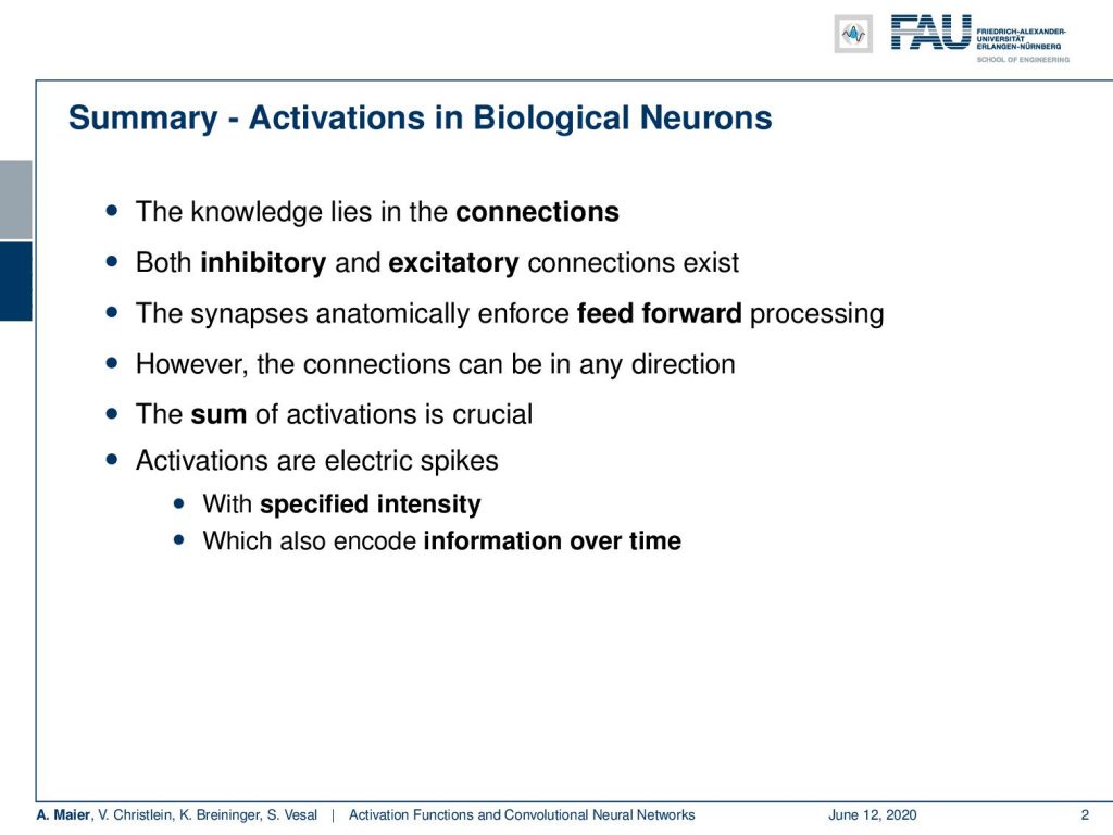
So, what we can see is the knowledge essentially lies in the connections between the neurons. We have both inhibitory and excitatory connections. The synapses anatomically enforce feed-forward processing. So, it’s very similar to what we’ve seen so far. However, those connections can be in any direction. So, they can also form cycles and you have entire networks of neurons that are connected with different axons in order to form different cognitive functions. Crucial is the sum of activations. Only if the sum of activations is above the threshold, then you will actually end up with an activation. These activations are electric spikes with a specified intensity and to be honest, the whole system is also time-dependent. Hence, they also encode the entire information over time. So, it’s not just that we have a single event that passes through but the whole process runs at a certain frequency. This enables the entire processing over time.
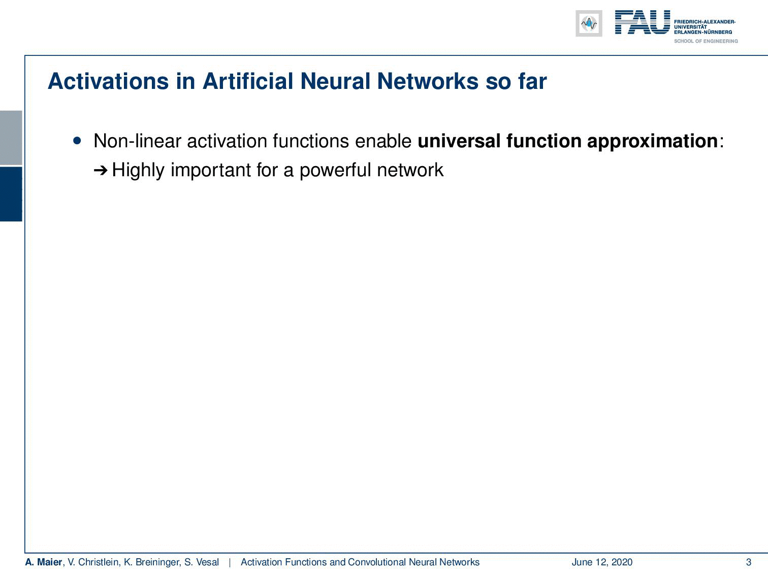
Now, activations in artificial neural networks so far they were nonlinear activation functions and mainly motivated by the universal function approximation. So if we don’t have the nonlinearities, we can’t get a powerful network. Without the nonlinearities, we would just end up with matrix multiplication. So compared to biology, we have some sign function that can model all-or-nothing responses. Generally, our activations have no time component. Maybe, this could be modeled by the activation strength of the sign function. Of course, it is also mathematically undesirable because the derivative of the sine function is zero everywhere except at zero where we have infinity. So this is absolutely not suited for backpropagation. Hence, we’ve been using the sigmoid function because we can compute an analytic derivative. Now the question is “Can we do better?”.
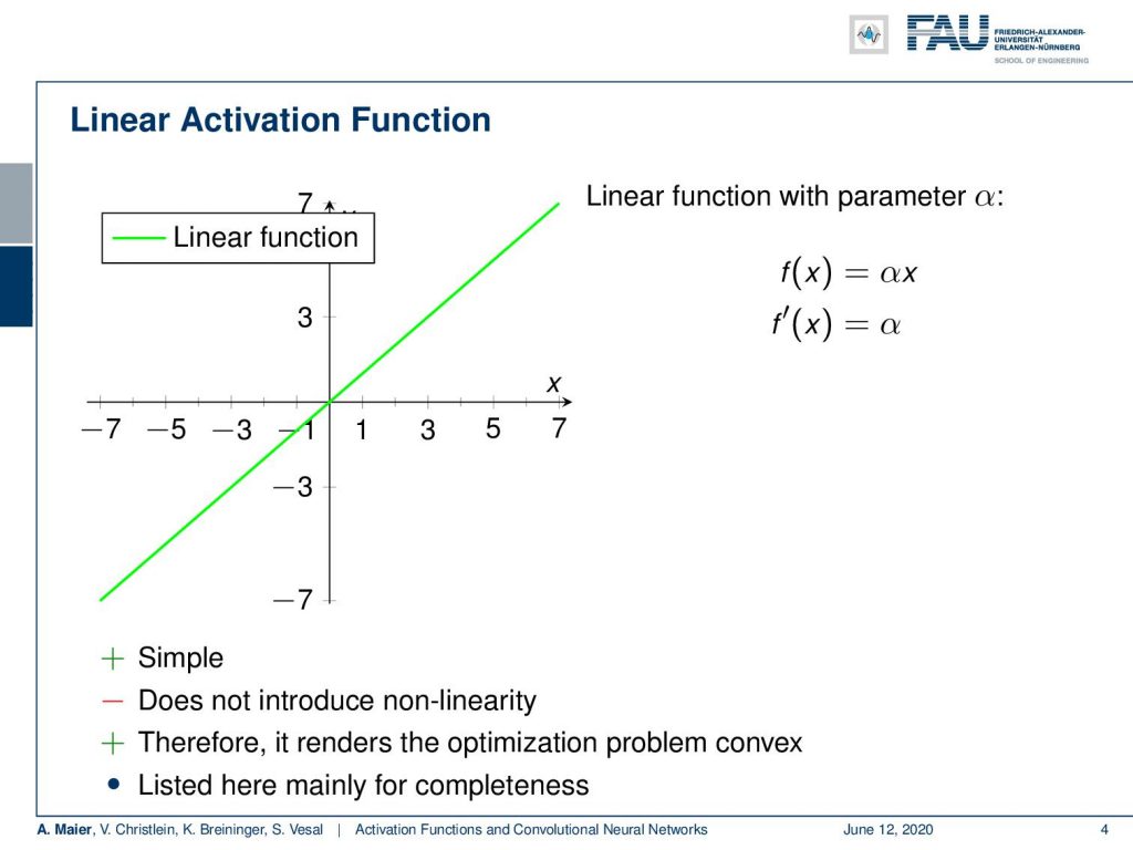
So, let’s look at some activation functions. The most simple one that we can think of is a linear activation where we just reproduce the input. We may want to scale it with some parameter α and then get the output. If we do, so we get a derivative of α. It’s very simple and it would render the entire optimization process into a convex problem. If we don’t introduce any non-linearity, we are essentially stuck with matrix multiplications. As such, we only list it here for completeness. It would not allow you to build deep neural networks as we know them.
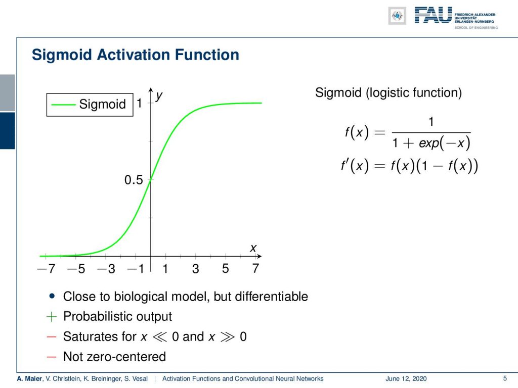
Now, the sigmoid function is the first one that we started with. It essentially has a saturation towards 1 and 0. So, it has a probabilistic output which is very nice. However, it saturates for x going towards very large or very low values. You can see here that the derivative already around 3 or -3 is approaching zero very quickly. Another problem is that it’s not zero centered.
Well, the problem of the zero centering is that you always produce positive numbers independent of what input you get. Your output will always be positive because we map towards values between 0 and 1. This means that if we had a signal of zero mean as input into this activation function, it will always be shifted towards a mean that will be greater than zero. This is called the internal covariate shift of successive layers. So, the layers constantly have to adapt to the shifting distribution. As a result, batch learning reduces the variance of the updates.
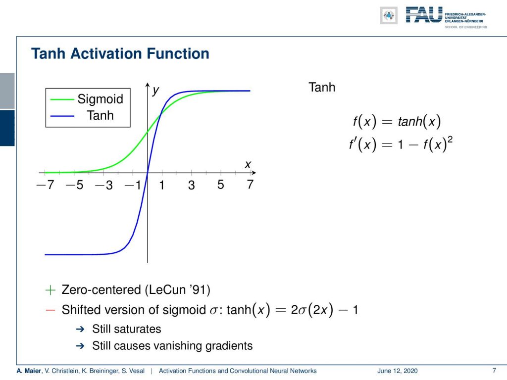
So what can we do in order to compensate for this? Well, we can work with other activation functions and a very popular one is the tangens hyperbolicus. It is shown here in blue. You can see that it has very nice properties. For example, it’s zero centered and has already been used by LeCun since 1991. So, you could say it’s a shifted version of the sigmoid function. But one main problem of course remains. This is saturation. So you can see that maybe at 2 or -2, you already see that the derivatives are very close to zero. So it still causes the vanishing gradient problem.
Well, now the essence here is how does x affect y. Our sigmoid and hyperbolic tangent, they map large regions of x to very small regions in y. So, this means that large changes in x will result in minimal changes in y. So, the gradient vanishes. The problem is amplified by backpropagation where you have many steps of very small numbers. If they are close to zero and you multiply those updates steps with each other, you get an exponential decay. The deeper you build the network, the faster the gradient vanishes, and the more difficult it is to update the lower layers. So, a very related problem is of course the exploding gradient. So, here we had the problem that we have high values and those high values amplify each other. As a result, we get an exploding gradient.
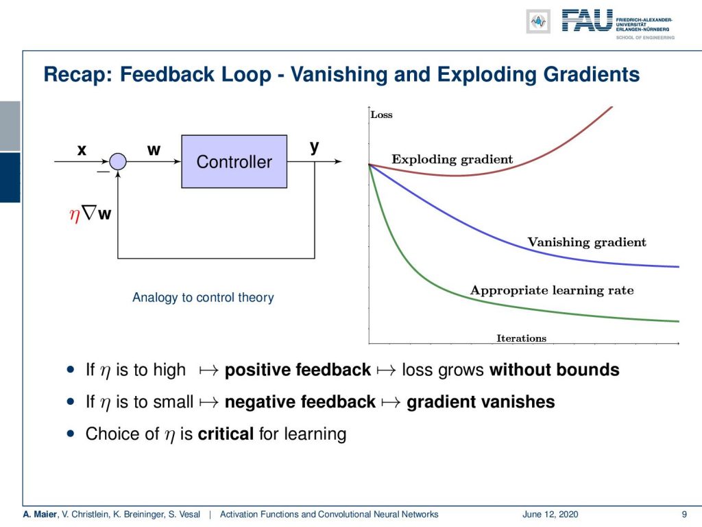
So, we can think about our feedback loop and the controller that we’ve seen before. We have seen what will happen with your lost curve if you measure the loss over the training iterations. If you don’t adjust the learning rates appropriately, you get exploding gradients or the vanishing gradients. But it’s not just the learning rate η. The problem can also be amplified by the activation functions. In particular, the vanishing gradient is a problem that occurs with those saturating activation functions. So we might want to think about that and see whether we can get better activation functions.
So next time on deep learning, we’ll exactly look at those activation functions. What you’ve seen today are essentially the classical ones and in the next session, we’ll talk about the improvements that have been done in order to build much more stable activation functions. This will enable us to go into really deep networks. Thank you very much for listening and see you in the next session!
If you liked this post, you can find more essays here, more educational material on Machine Learning here, or have a look at our Deep Learning Lecture. I would also appreciate a clap or a follow on YouTube, Twitter, Facebook, or LinkedIn in case you want to be informed about more essays, videos, and research in the future. This article is released under the Creative Commons 4.0 Attribution License and can be reprinted and modified if referenced.
References
[1] I. J. Goodfellow, D. Warde-Farley, M. Mirza, et al. “Maxout Networks”. In: ArXiv e-prints (Feb. 2013). arXiv: 1302.4389 [stat.ML].
[2] Kaiming He, Xiangyu Zhang, Shaoqing Ren, et al. “Delving Deep into Rectifiers: Surpassing Human-Level Performance on ImageNet Classification”. In: CoRR abs/1502.01852 (2015). arXiv: 1502.01852.
[3] Günter Klambauer, Thomas Unterthiner, Andreas Mayr, et al. “Self-Normalizing Neural Networks”. In: Advances in Neural Information Processing Systems (NIPS). Vol. abs/1706.02515. 2017. arXiv: 1706.02515.
[4] Min Lin, Qiang Chen, and Shuicheng Yan. “Network In Network”. In: CoRR abs/1312.4400 (2013). arXiv: 1312.4400.
[5] Andrew L. Maas, Awni Y. Hannun, and Andrew Y. Ng. “Rectifier Nonlinearities Improve Neural Network Acoustic Models”. In: Proc. ICML. Vol. 30. 1. 2013.
[6] Prajit Ramachandran, Barret Zoph, and Quoc V. Le. “Searching for Activation Functions”. In: CoRR abs/1710.05941 (2017). arXiv: 1710.05941.
[7] Stefan Elfwing, Eiji Uchibe, and Kenji Doya. “Sigmoid-weighted linear units for neural network function approximation in reinforcement learning”. In: arXiv preprint arXiv:1702.03118 (2017).
[8] Christian Szegedy, Wei Liu, Yangqing Jia, et al. “Going Deeper with Convolutions”. In: CoRR abs/1409.4842 (2014). arXiv: 1409.4842.