Lecture Notes in Deep Learning: Loss and Optimization – Part 3

Optimization with ADAM and beyond…

These are the lecture notes for FAU’s YouTube Lecture “Deep Learning“. This is a full transcript of the lecture video & matching slides. We hope, you enjoy this as much as the videos. Of course, this transcript was created with deep learning techniques largely automatically and only minor manual modifications were performed. If you spot mistakes, please let us know!

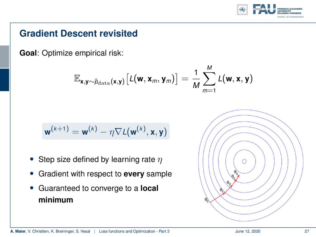
Welcome everybody to our next lecture on deep learning! Today, we want to talk about optimization. Let’s have a look at the gradient descent methods in a little bit more detail. So, we’ve seen that the gradient is essentially optimizing the empirical risk. Here in this figure, you see that we do one step each towards this local minimum. We have this predefined learning rate η. So, the gradient is of course computed with respect to every sample and this is then guaranteed to converge to a local minimum.

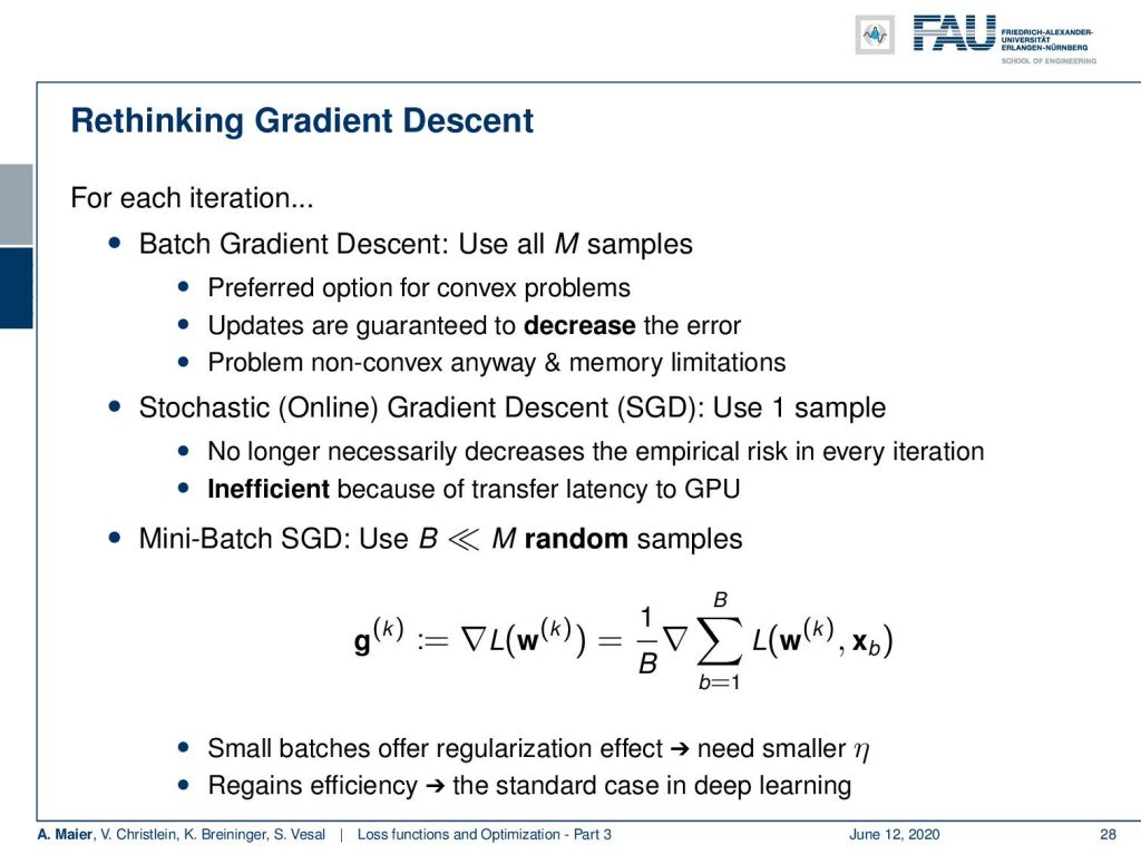
Now, of course, this means that for every iteration, we have to use all samples and this is called batch gradient descent. So you have to look in every iteration, for every update, at all samples. It may be really many samples, in particular if you look at big data a computer vision problems. This is of course a preferred option for convex optimization problems because we have a guarantee here that we find the global minimum. Every update is guaranteed to decrease the error. Of course, for non-convex problems, we have a problem anyway. Also, we may have memory limitations. This is why people like to prefer other approaches like the stochastic gradient descent SGD. Here, they use just one sample and then immediately update. So, this is no longer necessarily decreasing the empirical risk in every iteration and it may also be very inefficient because of the latency in transfers to the graphical processing unit. However, if you use just one sample you can do many things in parallel so it’s highly parallelizable. A compromise between the two is that you can use Mini-Batch stochastic gradient descent. Here you use B and B may be a number much smaller than the entire training data set of random samples that you essentially choose them randomly from the entire training data set. Then, you evaluate the gradient on the subset B. This is then called a mini-batch. Now, this mini-batch can be evaluated really quickly and you may also use parallelization approaches and because you can do several mini-batch steps in parallel. Then, you just do the weighted sum and update. So, small batches are useful because they offer a kind of regularization effect. This then typically results in smaller η. So, you have if you use a mini-batch in gradient descent, typically smaller values of η are sufficient and it also regains efficiency. Typically, this is the standard case in deep learning.

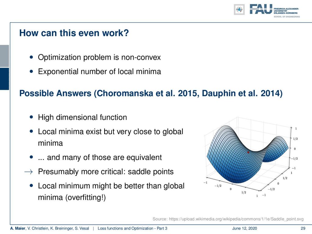
So, a lot of people work with this, meaning that the gradient descent is effective. But the question is: “How can this even work?” Our optimization problem is non-convex. There’s an exponential number of local minima and there’s an interesting paper from 2015 and where they show that the metrics that we are typically working with are high dimensional functions. There are many local minima in this environment. The interesting thing is that those local minima are close to the global minimum and actually many of those are equivalent. What is probably more of a problem are saddle points. Also, the local minima might even be better than the global minimum because the global minimum is attained on your training set, but in the end, you want to apply your network to a test data set that may be different. Actually, a global minimum on your training data set may be related to an overfit. Maybe, this is even worse for the generalization of the trained network.

One more possible answer to this is a paper from 2016. The authors are suggesting over-provisioning as there are many different ways of how a network can approximate the desired relationship. You essentially just need to find one. You don’t need to find all of them. A single one is sufficient. Liang at al. verified this experimentally by experiments with random labels. Here, the idea is that you essentially randomize the labels you don’t use the original. You just randomly assign any classes and if you then show that your experiment still solves the problem, then you are creating an overfit.

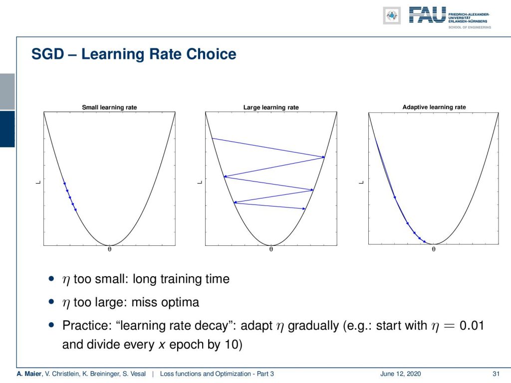
Let’s have a look at the choice of η. What we’ve already seen that if you have a small learning rate, we may stop even before we reach convergence. If you have a too large learning rate, we might be ending jumping back and forth and not even finding the local minimum. Only with an appropriate learning rate, you will be able to find the minimum. Actually, when you’re far away from the minimum, you want to be able to make big steps, and the closer you get to the minimum smaller steps. If you want to do so in practice, you work with the decay of the learning rate. So, you adapt your η gradually. You start with let’s say 0.01 and then you divide by ten every x epochs. This helps that you don’t miss the local minimum that you’re actually looking for. It’s a typical practical engineering parameter.

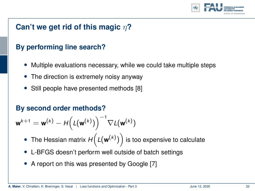
Now, you may ask can’t we get rid of this magic η? So what is typically done? Quite a few people suggest doing a line search in similar cases. So, line search of course needs you to estimate the optimal η at every step. So, you need multiple evaluations in order to find the correct η in the direction that the gradient points. It is extremely noisy anyway. So, people have presented methods but they are not the state of the art right now in deep learning. Then, people have suggested second-order methods. If you look into second-order methods, you need to compute the Hessian matrix and this is typically very expensive to calculate. So far, we have not seen that too often. There are L-BFGS methods but they typically don’t perform very well if you are operating outside of the batch setting. So, if you work with mini-batches, they are not that great. There’s a report on that by Google that you can find in reference [7].

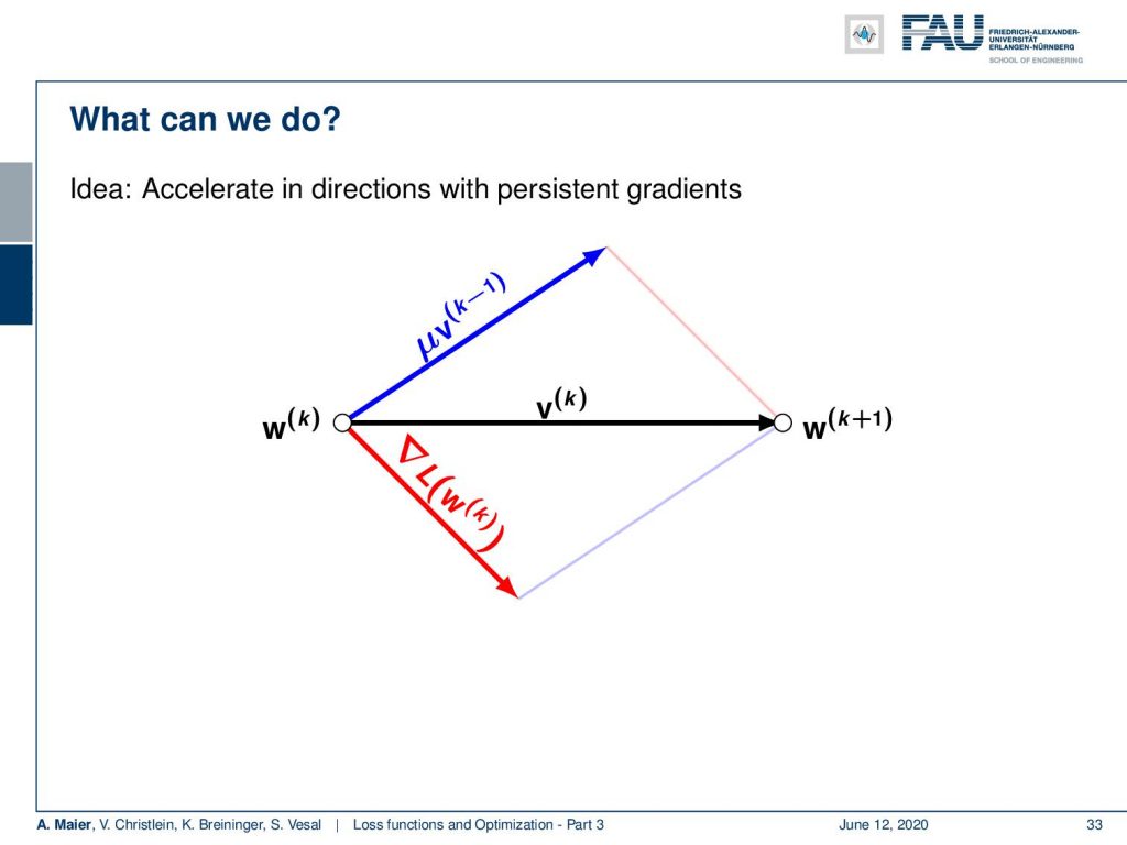
What else can we do? Well, of course, we could accelerate the directions of persistent gradients. So, the idea here would be that you somehow keep track of the average that is indicated here with new v. This is essentially a weighted sum over the last couple of gradient steps. You take the current gradient direction indicated in red and average it with the previous steps. This then gives you an updated direction and this is typically called a momentum.

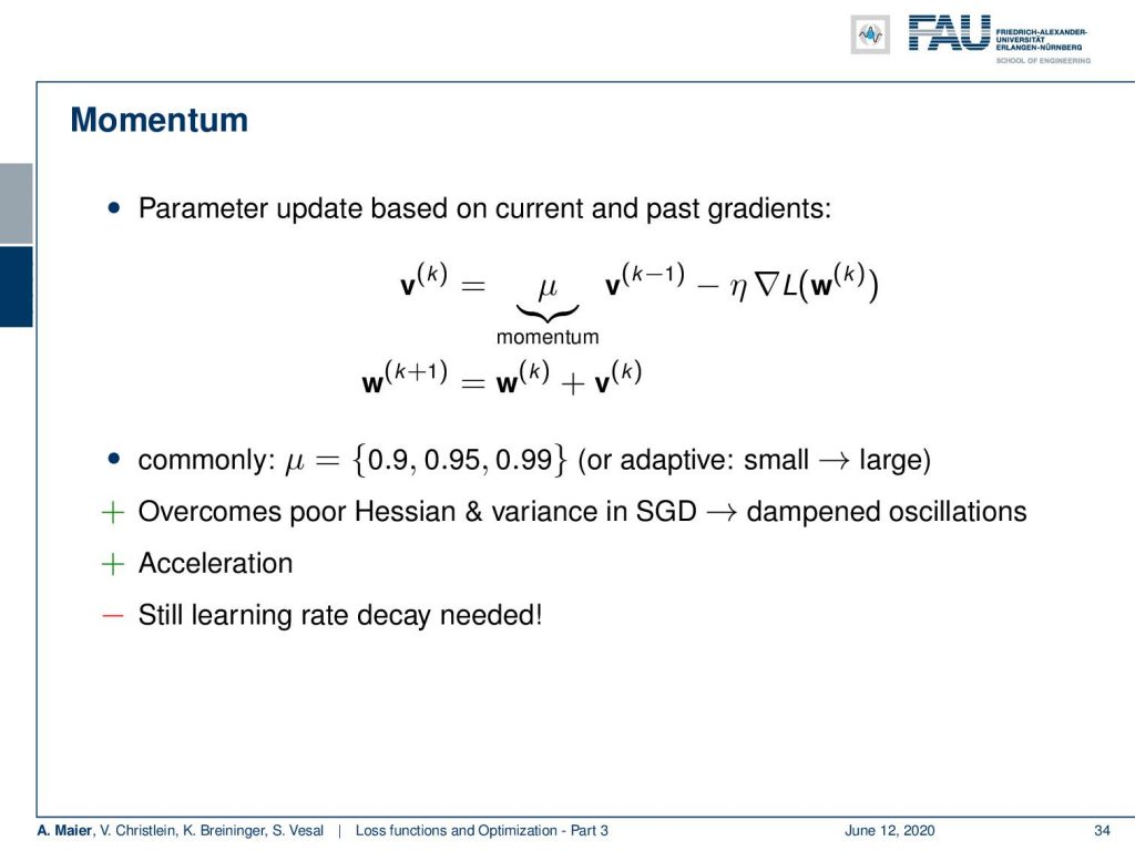
So, we introduce this momentum term. There you add with a new weight some momentum that is indicated with v superscript k-1. This momentum term is essentially computed in an iterative fashion where you iteratively update over the past gradient directions. So you can essentially say by iteratively computing this weighted mean, you keep a history of the previous gradient directions and you gradually update them with the new gradient direction. Then you pick the momentum term in order to perform the update instead of just the gradient direction. So, typical choices for μ are 0.9, 0.95, or 0.99. You can also adapt them from small to large if you want them to pay more emphasis on the previous gradient directions. This overcomes poor Hessians and variance in the stochastic gradient descent. It will dampen oscillations and it accelerates typically the optimization procedures. Still, we need the learning rate decay. So, this doesn’t solve the automatic adjustment of η.

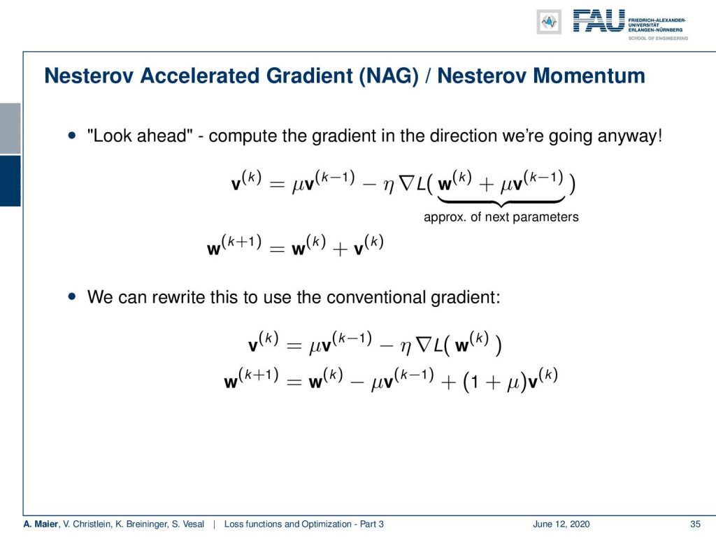
We can also pick a different way of momentum: the Nesterov Accelerated Gradient or simply Nesterov Momentum. This performs a look-ahead. So here, we also have this momentum term. But instead of evaluating the gradient at the position we’re currently at, we add the momentum term before computing the gradient. So, we are essentially trying to approximate the next set of parameters. We use the look-ahead it here and then we perform the gradient update. So you can rewrite this to use the conventional gradient. The idea here is to put the Nesterov Acceleration directly into the gradient update. This term will then be used in the next gradient update. So, this is an equivalent formulation.

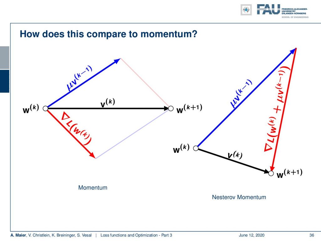
Let’s visualize this a bit. Here, you can see momentum and the Nesterov Momentum. Of course, they both use a kind of momentum term. But they use a different direction for calculating the gradient update. That’s the main difference.

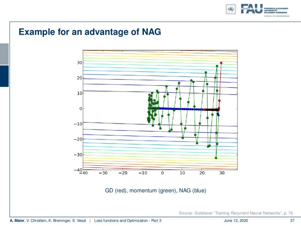
Here, you see an example of these momentum terms in comparison. In this situation, you have a strong disagreement in the variance in both directions. So, we have a very high variance in left and right directions and a rather small variance in the top-bottom direction. We’re trying to find the global minimum. This then leads typically to alternating gradient directions very strongly even if you introduce the momentum term. You still get this strong oscillating behavior. If you use the Nesterov Accelerated Gradient, you can see that we compute this look-ahead and this allows us to follow the blue line. So, we are directly moving towards the desired minimum and we are no longer alternating. This is an advantage of Nesterov.

What if our features have different needs? So, suppose some features are activated very infrequently while others are updated very often. Then, we would need individual learning rates for every parameter in the network. We need large learning rates for infrequent parameters and small learning rates for frequent parameters.

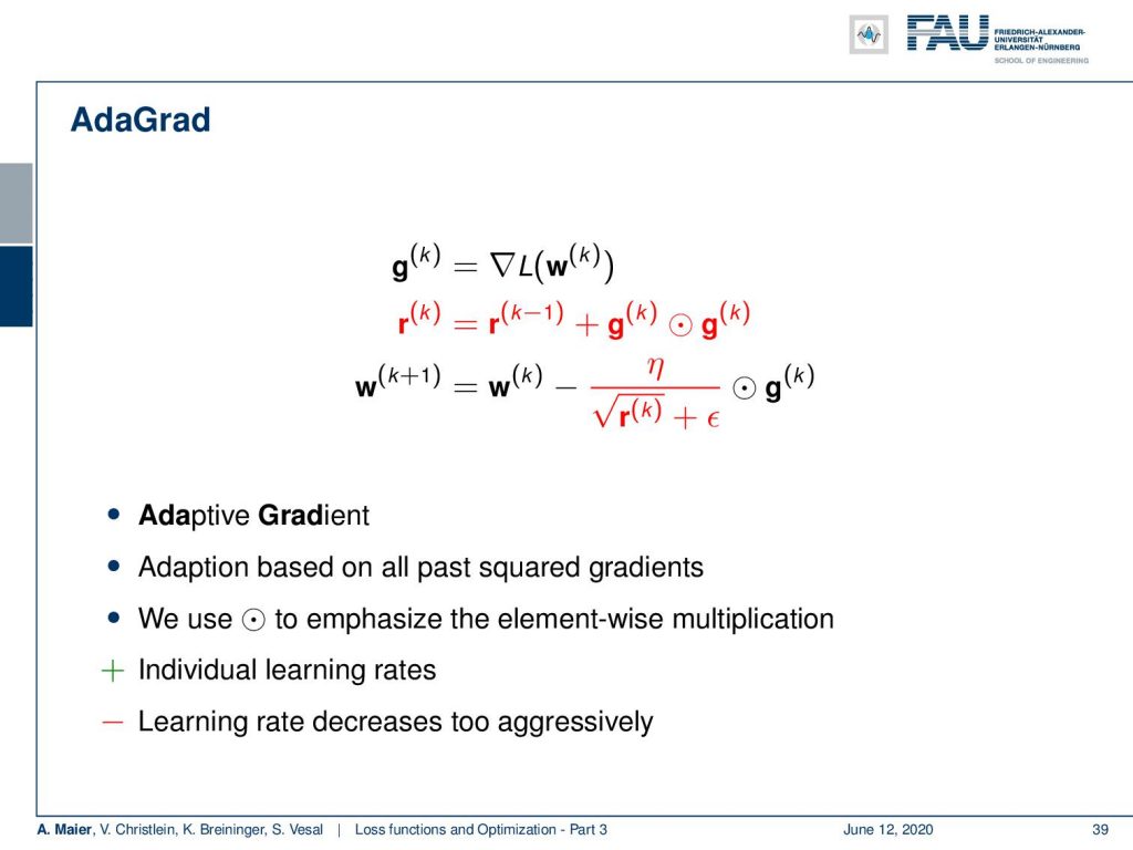
In order to accommodate the changes appropriately, this can be done with the so-called AdaGrad method. It is using first the gradient to compute some g superscript k and then it’s computing the product of the gradient with itself to keeps track of its element-wise variance in a variable r. Now, we use our g and our r elementwise as in combination with η to weigh the update of the gradient. So, now we construct updated weights and the variance of the weights in every parameter is incorporated by multiplying with the square root of the respective element, i.e. an approximation of its standard deviation. So, here we note this down as a square root of an entire vector. All the other things here are scalar which means that this also results in a vector again. This vector is then multiplied point-wise with the actual gradient to perform a local scaling. It’s a nice and efficient method and allows individual learning rates for all of the different dimensions for all of the different weights. One problem could be that the learning rate decreases too aggressively.

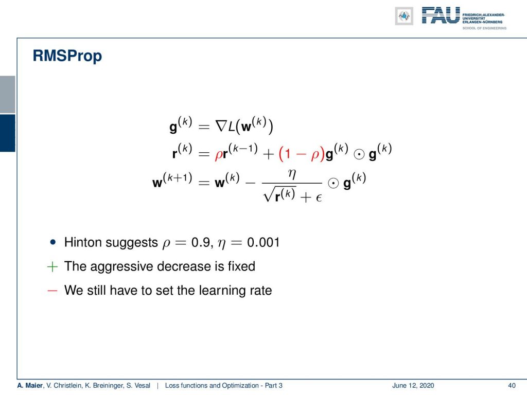
This is a problem and leads to an improved version and the improved version here is RMSProp. RMSProp is now using this again, but they introduce this ρ and now ρ is being used to essentially introduce a delay such that you don’t have very high increases. Here you can set this ρ in order to dampen the update of the variance of the learning rate. So, Hinton suggests 0.9 and η = 0.001. This turn leads to the aggressive decrease being fixed, but we still have to set the learning rate. If you don’t set the learning rate appropriately, you run into a problem.

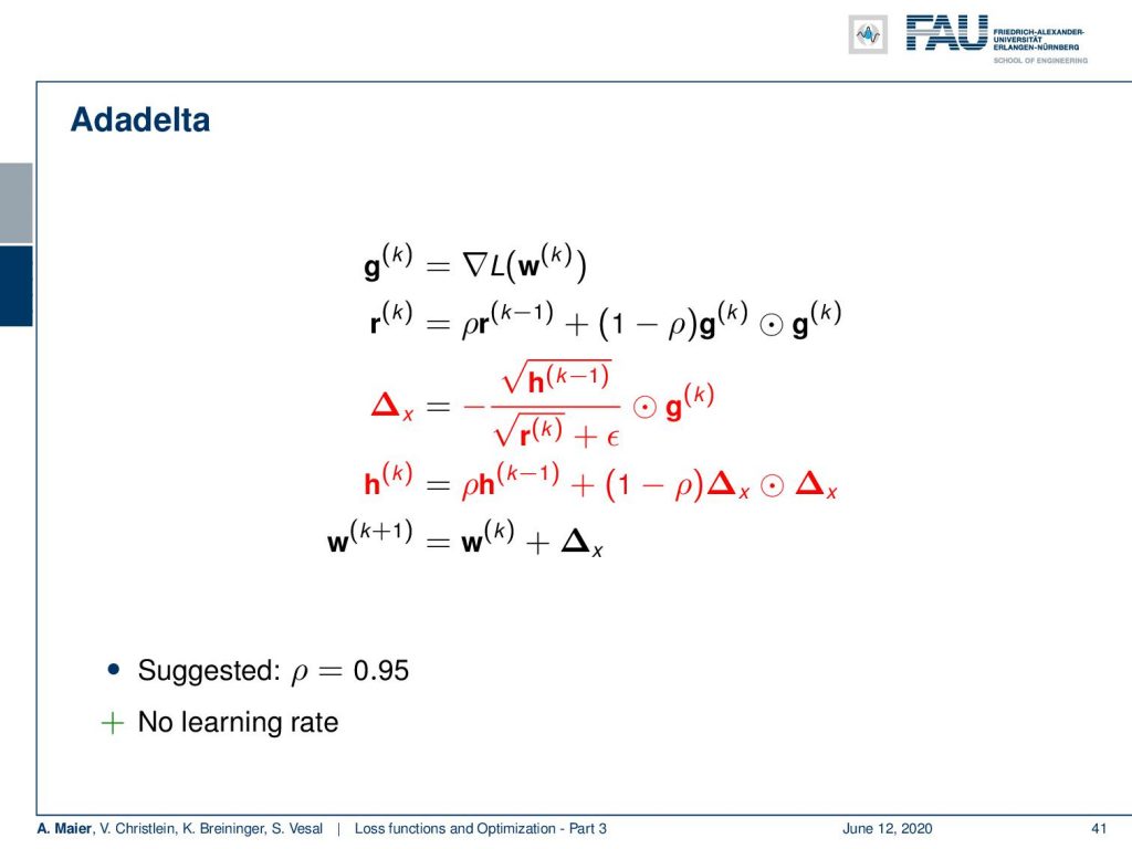
Now, Adadelta tries to improve on this further. They use essentially our RMSProp and get rid of η. So, we already have seen r. It is the variance that is computed in a dampened way. Then, in addition, they introduce this Δₓ. It is a weighted combination of some term h and the r that we have seen previously multiplied to the gradient direction. So, this is an additional dampening factor that replaces the η in the original formulation. The factor h is computed again as a sliding average over the Δₓ as an element-wise product. So, this way you don’t have to set a learning rate anymore. Still, you have to choose the parameter ρ. For ρ we suggest going to 0.95.

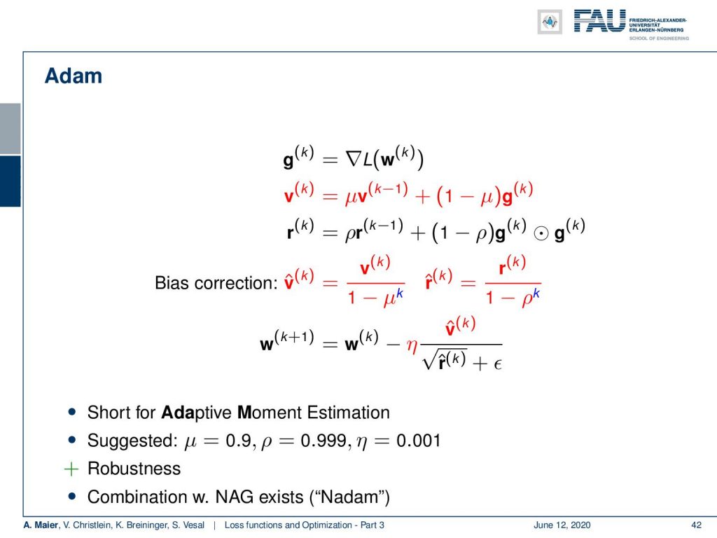
One of the most popular algorithms that are being used is Adam and Adam is essentially also using this gradient direction g. Then, you have essentially a momentum term v. In addition, you have this r term that is again trying to steer the learning rate for each dimension individually. Furthermore, Adam introduces an additional bias correction where v is scaled by 1 minus μ. r is also scaled by 1 over 1 minus ρ. This then leads to the final update term that involves the learning rate η, our momentum term, and the respective scaling. This algorithm is called Adaptive Moment estimation. For Adam suggested values are μ = 0.9, ρ = 0.999 and η=0,001. It’s a very robust method and very commonly used. We can combine it with the Nesterov accelerated gradient and you get “Nadam”. But still, you can improve on this.

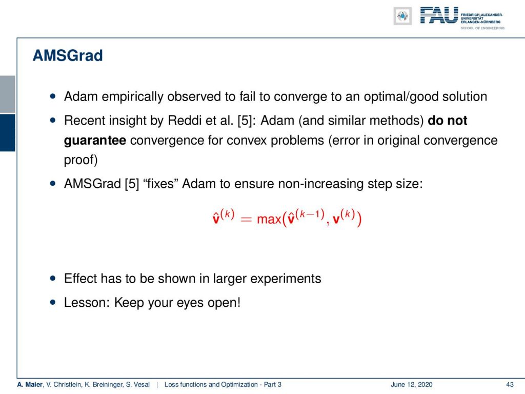
Adam was empirically observed to fail to converge to optimal/good solutions. In reference [5], you can even see that Adam and similar methods do not guarantee to converge for convex problems. There’s an error in the original convergence proof and therefore, we suggest using AMSGrad that fixes Adam to ensure non increasing step size. So, you can fix it by adding a maximum over the momentum update term. So if you do this, you result in AMSGrad. This is shown to be even more robust. The effect has been shown in large experiments. One lesson that we learn here is that you should keep your eyes open. Even things that go through scientific peer review may have problems that are later identified. Another thing that we learned here is that these gradient descent procedures – as long as you approximately follow the correct gradient direction – you still get quite decent results. Of course, such gradient methods are really hard to debug. So, be sure that you debug your gradients. This really happens as you can see in this example. Even large software frameworks may suffer from such errors. For a long time, people didn’t notice them. They just notice strange behavior, but the problem persists.

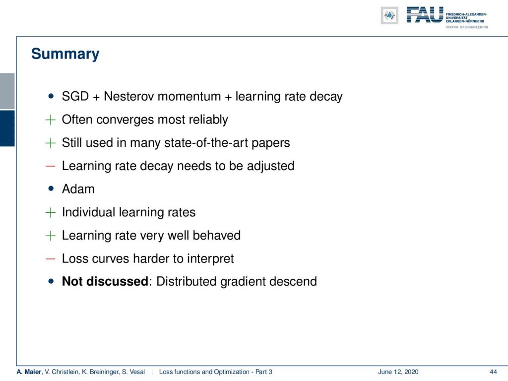
Okay, so let’s summarize this a bit. The stochastic gradient descent plus Nesterov momentum plus learning rate decay is a typical choice in many experiments. It converges most reliably and is used in many state-of-the-art papers. Still, it has the problem that this learning rate decay has to be adjusted. Adam has individual learning rates. The learning rates are very well-behaved, but of course, the loss curves are much harder to interpret because you don’t have this typical behavior as you would see with fixed learning rates. What we didn’t discuss here and we only hinted at that is distributed gradient descent. Of course, you can also do this in a parallelized manner and then compute different update steps in different nodes of a distributed network or on different graphic boards. Then you average over them. This has also been shown to be very robust and very fast.

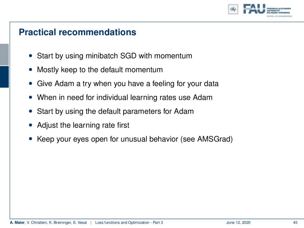
Some practical recommendations: Start by using mini-batch stochastic gradient descent with momentum. Stick to the default momentum. Give Adam a try when you have a feeling for your data. When you see that you need individual learning rates then Adam can help you with getting better or more stable convergence. You can also switch to AMSGrad which is an improvement over Adam. Of course, start adjusting the learning rate first and then keep your eyes open regarding unusual behavior.

Okay, this brings us to a short outlook on the next couple of videos and what we are coming up with. Of course the actual deep learning part, we haven’t discussed this at all so far. So one problem that we still need to talk about is how can we deal with spatial correlation and features. We hear so much about convolution and neural networks. Next time we see why this is a good idea how is it implemented. Of course, one thing that we should think about is how to use variances and how to incorporate them into network architectures.

Some comprehensive questions: “What are our standard loss functions for classification and regression?” So of course, L2 for regression and cross-entropy loss for classification. You should be able to derive those. This is really something that you should know because the statistics and their relations to learning losses are really important. The statistical assumptions, probabilistic theory, and how to modify those to get to our loss functions are highly relevant for the exam. Very important are also subdifferentials. “What’s a subdifferential?” “How can we optimize in situations where our activation functions have a kink?” “What’s the hinge loss?” “How can we incorporate constraints?” and in particular “What do we tell people that claim that all our techniques are not good because an SVM is superior?” Well, you can always show that it’s up to a multiplicative constant the same as using hinge loss. “What is Nesterov Momentum?” These are very typical things you should be able to explain if somebody in the near future is going to ask you questions about the things that you have been learning here. Of course, we have plenty of references again (see below). I hope you enjoyed this lecture as well and I am looking forward to seeing you in the next one!

If you liked this post, you can find more essays here, more educational material on Machine Learning here, or have a look at our Deep Learning Lecture. I would also appreciate a clap or a follow on YouTube, Twitter, Facebook, or LinkedIn in case you want to be informed about more essays, videos, and research in the future. This article is released under the Creative Commons 4.0 Attribution License and can be reprinted and modified if referenced.

References

[1] Christopher M. Bishop. Pattern Recognition and Machine Learning (Information Science and Statistics). Secaucus, NJ, USA: Springer-Verlag New York, Inc., 2006.
[2] Anna Choromanska, Mikael Henaff, Michael Mathieu, et al. “The Loss Surfaces of Multilayer Networks.” In: AISTATS. 2015.
[3] Yann N Dauphin, Razvan Pascanu, Caglar Gulcehre, et al. “Identifying and attacking the saddle point problem in high-dimensional non-convex optimization”. In: Advances in neural information processing systems. 2014, pp. 2933–2941.
[4] Yichuan Tang. “Deep learning using linear support vector machines”. In: arXiv preprint arXiv:1306.0239 (2013).
[5] Sashank J. Reddi, Satyen Kale, and Sanjiv Kumar. “On the Convergence of Adam and Beyond”. In: International Conference on Learning Representations. 2018.
[6] Katarzyna Janocha and Wojciech Marian Czarnecki. “On Loss Functions for Deep Neural Networks in Classification”. In: arXiv preprint arXiv:1702.05659 (2017).
[7] Jeffrey Dean, Greg Corrado, Rajat Monga, et al. “Large scale distributed deep networks”. In: Advances in neural information processing systems. 2012, pp. 1223–1231.
[8] Maren Mahsereci and Philipp Hennig. “Probabilistic line searches for stochastic optimization”. In: Advances In Neural Information Processing Systems. 2015, pp. 181–189.
[9] Jason Weston, Chris Watkins, et al. “Support vector machines for multi-class pattern recognition.” In: ESANN. Vol. 99. 1999, pp. 219–224.
[10] Chiyuan Zhang, Samy Bengio, Moritz Hardt, et al. “Understanding deep learning requires rethinking generalization”. In: arXiv preprint arXiv:1611.03530 (2016).

Category: Lecture Notes in Deep Learning