
Do SVMs beat Deep Learning?
These are the lecture notes for FAU’s YouTube Lecture “Deep Learning“. This is a full transcript of the lecture video & matching slides. We hope, you enjoy this as much as the videos. Of course, this transcript was created with deep learning techniques largely automatically and only minor manual modifications were performed. If you spot mistakes, please let us know!
Welcome back to deep learning! So, let’s continue with our lecture. We want to talk about loss and optimization. Today, we want to talk a bit about loss functions and optimization. I want to look into a couple of more optimization problems and one of those optimization problems we’ve actually already seen in the perceptron case.
You remember that we were minimizing a sum over all of the misclassified samples. We were choosing this because we could somehow get rid of the sign function and only look into the samples that were relevant for misclassification. Also, note that here we don’t have a 0/1 category but a -1/1 because this allows us to multiply with the class label. This will then always result in a negative number in misclassified samples. Then we add this negative sign in the very beginning such that we always end up with a positive value. The smaller this positive value, the smaller our loss will be. So, we seek to minimize this function. We don’t have the sign function in this criterion because we found an elegant way to formulate this loss function without it. Now, if it were in we would run into problems because this would only count the number of misclassifications and we would not differentiate whether it’s far away from decision boundary or close to the decision boundary. We would simply end up with a count. If we look at the gradient, it would essentially vanish everywhere. So it’s not an easy optimization problem. We don’t know in which direction to go so we can’t find a good optimization. What did we do about this last time? Well, we somehow need to relax this and there are also ways how to fix this.
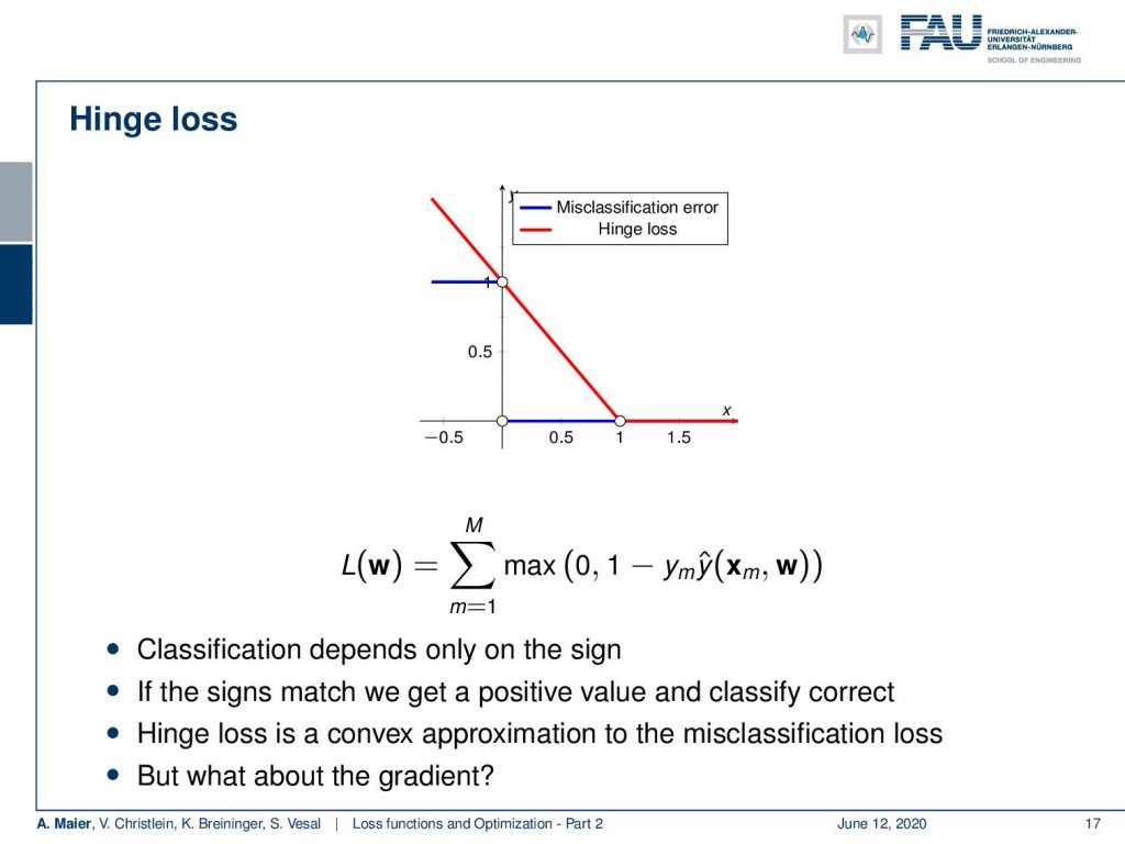
One way to go ahead is to include the so-called hinge loss. Now with the hinge loss, we can relax this 0/1 function into something that behaves linearly on a large domain. The idea is that we essentially use a line that hits the x-axis at 1 and the y-axis also at 1. If we do it this way, we can simply rewrite this using the max function. So, the hinge loss is then a sum over all the samples that essentially receive 0 if our value is larger than 1. So, we have to rewrite the right-hand part to reformulate this a little. We take 1 – y subscript m times y hat. Here, you can see that we will have the same constraint. If we have opposite sides of the boundary, this term will be negative and by the sign, it will of course be flipped such that we end up having large values for a high number of misclassifications. We got rid of the problem of having to find the set of misclassifications M. Now, we can take the full set of samples by using this max function because everything that will fulfill this constraint will automatically be clamped to 0. So, it will not influence this loss function. Thus, that’s a very interesting way of formulating the same problem. We get implicitly the situation that we only consider the misclassified samples in this loss function. It can be shown that the hinge loss is a convex approximation of the misclassification loss that we considered earlier. One big thing about this kind of optimization problem is of course the gradient. This loss function here has a kink. Thus, the derivative is not continuous in the point x = 1. So there it’s unclear what the derivative is and now you could say: “Okay, I can’t compute the derivative of this function. So, I’m doomed!”
Luckily subgradients save the day. So let’s introduce this concept and in order to do so, we have a look at convex differentiable functions. On those, we can say that at any point f(x), we can essentially find a lower bound of f(x) that is indicated by some f(x₀) plus the gradient at f(x₀) multiplied with the difference from x to x₀. So, let’s look at a graph to show this concept. If you look at this function here, you can see that I can take any point x₀ and compute the gradient, or in this case, it’s simply the tangent that is constructed. By doing so, you will see that at any point of the tangent will be a lower bound to the entire function. It doesn’t matter where I take this point if I follow the tangent in the tangential direction, I’m always constructing a lower bound. Now, this kind of definition is much more suited for us.
So, let’s expand now on the gradient and go into the direction of subgradients. In subgradients, we define something which keeps this property but is not necessarily a gradient. So a vector g is a subgradient of a convex function f(x₀) if we have the same property. So, if we follow the subgradient direction, multiply it with the difference between x and x₀, then we always have a lower bound. The nice thing with this is that we essentially can relax the requirement of being able to compute a gradient. There could be multiple of those g‘s that fulfill this property. So, g is not required to be unique. The set of all of these subgradients is then called the subdifferential. So, the subdifferential is then a set of subgradients that all fulfill the property above. If f(x) is differentiable at x₀, we can simply say that the set containing all sub differentials is simply the set containing the gradient.
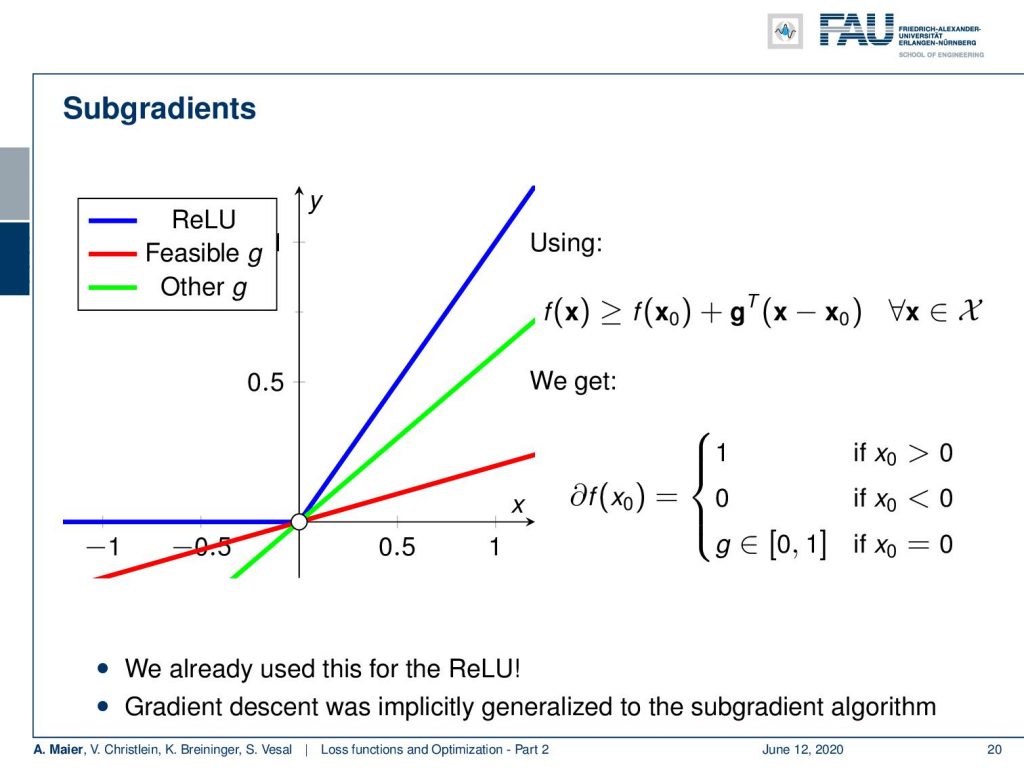
Now let’s look at a case where this is not true. In this example here, we have the rectified linear unit (ReLU) which also has exactly the same problem. Again it’s a convex function which means here at the point where we have the kink, we can find quite a few subgradients. Actually, you see the green line and the red line. Both of them are feasible subgradients and they fulfill this property that they are lower bounds to that respective function. So this means that we can now define a subdifferential and our subdifferential is essentially 1 where we have x₀ greater than 0. We have 0, where it’s smaller than 0. We have exactly g – and g can now be any number between 0 and 1 at the position x₀=0. This is nice because we can now follow essentially this subgradient direction. It’s just that the gradient is defined differently in different parts of the curve. In particular, at the kink position, we have this situation where we would have multiple possible solutions. But for our optimization, it’s sufficient to just know one of the subgradients. We don’t have to compute the entire set. So, we can now simply extend our gradient descent algorithm to generalize to subgradients. There are proofs that for convex problems, you will still find the global minimum using subgradient theory. So, we can now say: “Well, the functions that we are looking at, they are locally convex.” This then allows us to find the local minima even with ReLUs and with the hinge loss.
So, let’s summarize this a bit: Subgradients are a generalization of gradients for convex non-smooth functions. The gradient descent algorithm is replaced by the respective subgradient algorithm for these functions. Still, this allows us to continue essentially how we did before for piecewise continuous functions. You just choose a particular subgradient and you probably don’t even notice the difference. The nice thing is that we’re not just doing this as an “engineering solution”, but there is also a solid mathematical theory that this actually works. Hence, we can use this for our ReLU and our hinge loss. This is mathematically sound and we can go ahead and not worry too much.
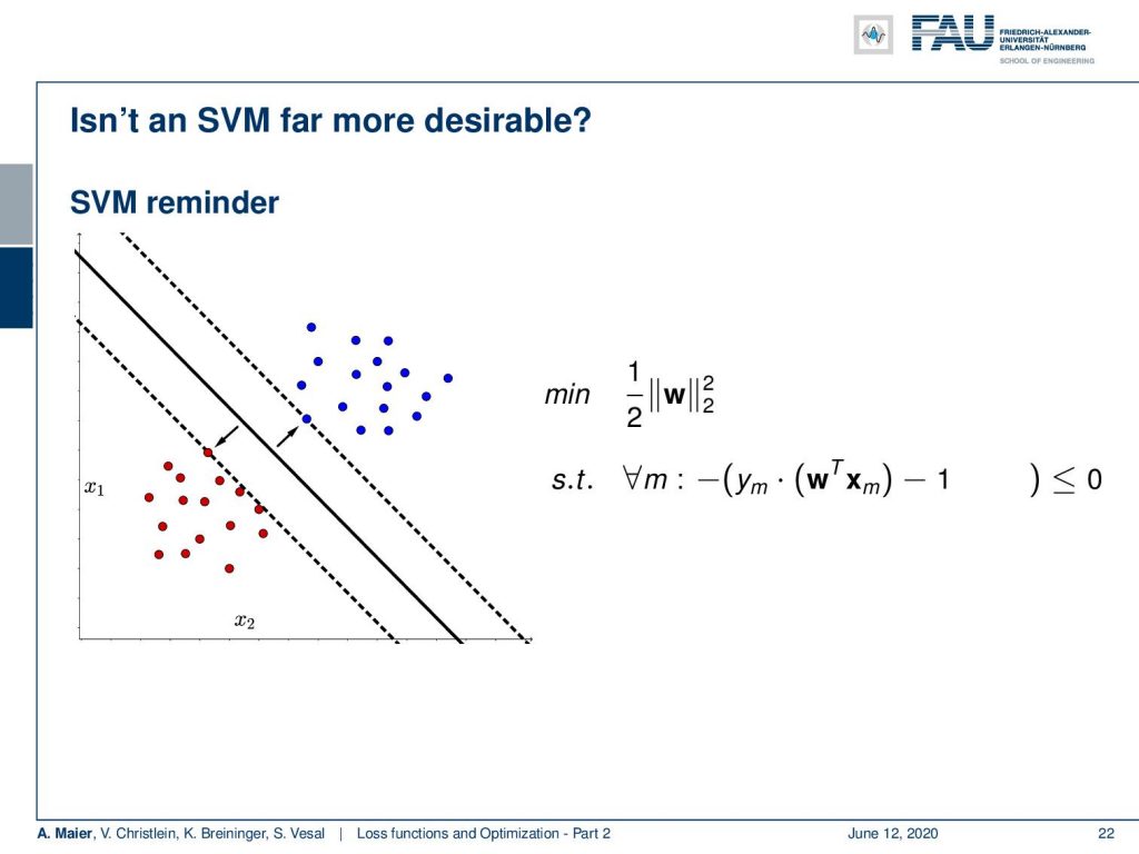
What if people say “Oh, Support Vector Machines (SVMs) are much better than what you’re doing, because they always achieve the global minimum.” So, isn’t it much better to use the SVM? So, let’s have a small look at what an SVM actually does. SVMs compute the optimally separating hyperplane. It’s also computing some plane that separates two classes with the idea is that it wants to maximize the margin between the two sets. So, you try to find the plane or here in this simple example, the line that produces the maximum margin. The hyperplane or the decision boundary is the black line and the dashed lines indicate the margin here. So, the SVM tries to find the margin that is maximally large while separating those classes. What is done typically is that you find this minimization problem where w is the normal vector of our hyperplane. We then minimize the magnitude of the normal vector. Note that this normal vector is not scaled which means that if you increase the magnitude of w, your normal vector gets longer. If you want to compute signed distances from that you typically divide by the magnitude of the normal vector. So, this means that if you increase the length of this normal vector your distances get smaller. If you want to maximize the distances, you minimize the length of the normal vector. Obviously, you could just collapse it to zero and then you would have essentially infinite distances. Just minimizing w would lead to the trivial solution w=0. To prevent this, you put this in a constraint optimization where you require for all observations m for all your samples that they are projected onto the right side of the decision boundary. This is introduced by this constraint minimization here. So you want to have the signed distance multiplied with the true label minus one to be smaller than 0.
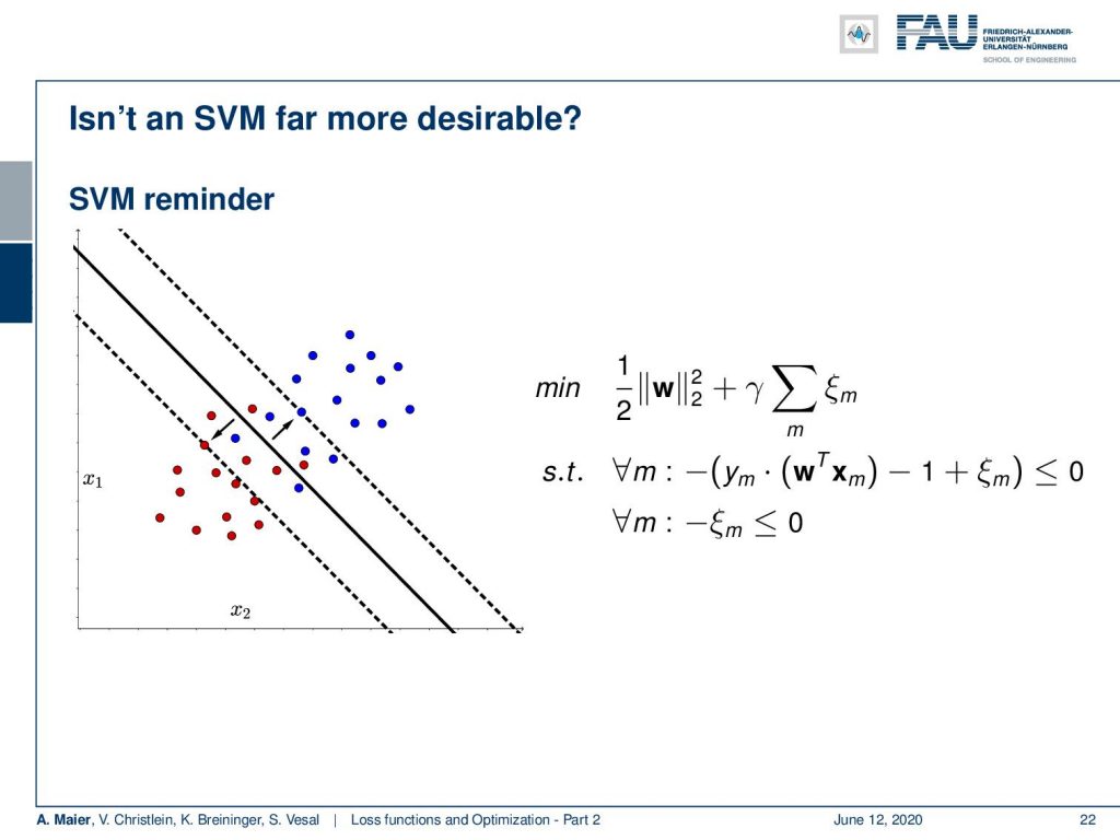
Now, we can expand this also to cases where the two classes are not linearly separable in the so-called soft margin SVM. The trick here that we introduce a slack variable ξ that allows a misclassification. ξ is added towards the distance to the decision boundary. This means that I can take individual points and move them back to the decision boundary if they were incorrectly classified. To limit excessive use of ξ, I postulate that the ξ are all smaller or equal to 0. Furthermore, I postulate that the sum over all the ξ needs to be minimized as I want to have as few misclassifications as possible.
This then leads us to the complete formulation of the soft margin SVM and if I want to do this in a joint optimization, you convert this to the Lagrangian dual function. In order to do so, you introduce Lagrange multipliers λ and ν. So, you can see that the constraints that we had in the previous slide, they now receive the multipliers λ and ν. Of course, there’s an additional new m that is introduced for the individual constraints. Now, you see that this forms a rather complex optimization problem. Still, we have a single Lagrangian function that can be sought to be minimized for all w, ξ, λ, and ν. So, there’s a lot of parameters introduced here. We can rearrange it a little bit and pull many of the parameters into one sum. If we drop the support vector interpretation, we can regard this sum as a constant. Because we know that all of the lambdas are larger or equal to 0, it means that everything that will be misclassified or is closer to the decision boundary than 1 will create a positive loss. If you replace the lambda term with the maximum function, you will get the same result. The optimization will always produce something that will be zero or greater in the case of misclassification or if you are inside the area of the margin. In this trick, we approximate this by introducing the max function to suppress everything that is below 0, i.e., on the correct side and outside of the margin. Now, you see that we can very elegantly express this as a hinge loss. So, you can show that the support vector machine and the hinge loss formulation with those constraints are equivalent up to an overall multiplicative constant as shown reference [1]. If people say: “Oh, you can’t do deep learning. Take an SVM instead!”. Well, if you choose the right loss function, you can also incorporate a support vector machine into your deep learning framework. That’s actually a quite nice observation.
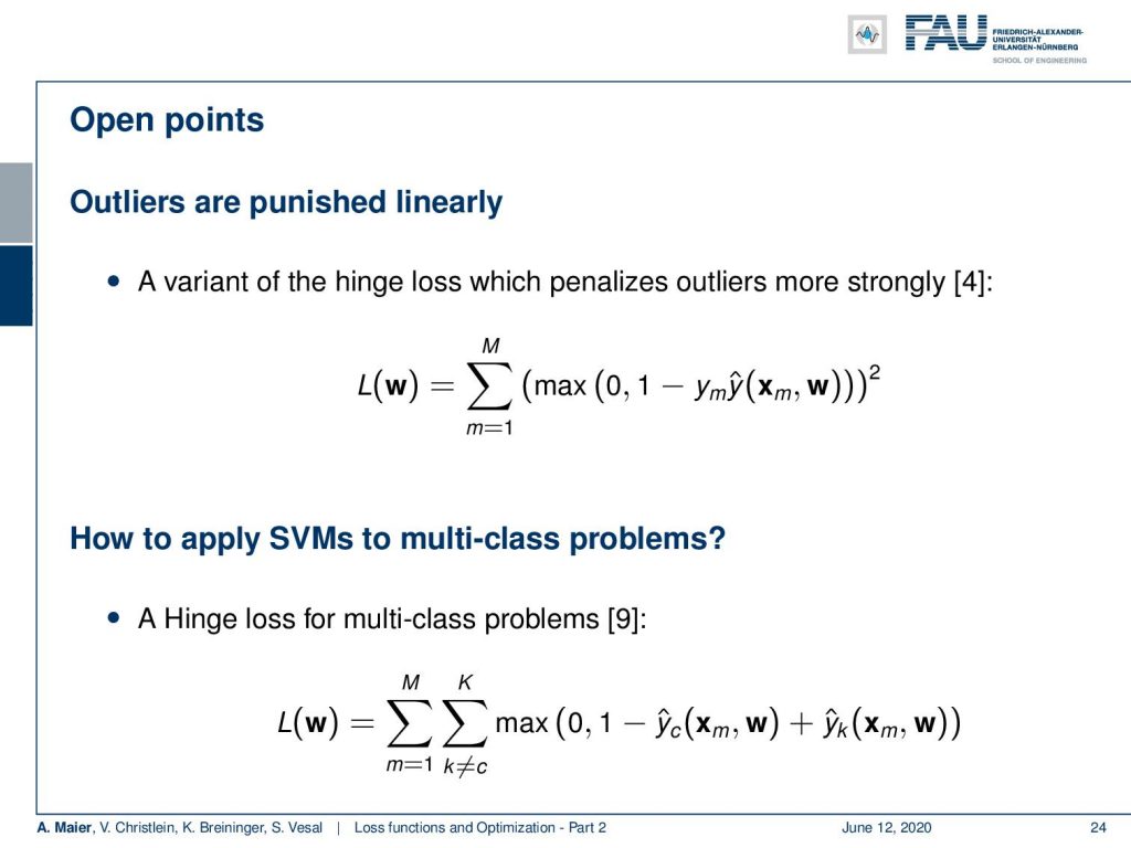
Okay some open points: Outliers are punished linearly. There’s a variant of the hinge loss which penalizes the outliers more strongly. You can do that for example by introducing squares. So also a very common choice see reference [4]. So, we can also apply this hinge loss to multi-class problems and what we are introducing here is simply an additional sum where we then do one versus many. So, we are not just classifying towards one class but we are classifying one versus the rest. This introduces the new classifiers shown here. In the very end, this leads to a multi-class hinge loss.
So, let’s summarize this a little bit: We have seen that we can incorporate SVMs into a neural network. We can do this with the hinge loss which is a loss function that you can put in all kinds of constraints in. You can even incorporate forced-choice experiments as a loss function. This has then been called user-loss. So it’s a very flexible function that allows you to formulate also all kinds of constrained optimization problems in the framework of deep learning. You can put all kinds of constrained optimization also into deep learning frameworks. Also very cool that you learned about subgradients and why we can deal with non-smooth objective functions. So this is also a very useful part and if you run into a mathematician and they tell you “Oh, there’s this kink and you can’t compute the gradient!”. So from now on, you say: “Hey, subgradients save the day!”. This way, we just need to find one possible gradient and then it still works. This is really nice. Check our references if somebody ever approaches you that ReLUs are not okay in your gradient descent procedure. There are proofs for that.
Next time in deep learning, we want to go ahead and look a bit into the optimization. So far, all the optimization programs that we considered, they just had this η and this was somehow doing the same for all variables. Now, we’ve seen that different layers parameters can be very different and maybe, then they should not be just treated all equally. Actually, this will lead to big trouble. But if you look into more advanced optimization programs, they have some cool solutions how to treat the individual weights differently automatically. So stay tuned! I hope you like this lecture and would love to welcome you again in the next video!
If you liked this post, you can find more essays here, more educational material on Machine Learning here, or have a look at our Deep Learning Lecture. I would also appreciate a clap or a follow on YouTube, Twitter, Facebook, or LinkedIn in case you want to be informed about more essays, videos, and research in the future. This article is released under the Creative Commons 4.0 Attribution License and can be reprinted and modified if referenced.
References
[1] Christopher M. Bishop. Pattern Recognition and Machine Learning (Information Science and Statistics). Secaucus, NJ, USA: Springer-Verlag New York, Inc., 2006.
[2] Anna Choromanska, Mikael Henaff, Michael Mathieu, et al. “The Loss Surfaces of Multilayer Networks.” In: AISTATS. 2015.
[3] Yann N Dauphin, Razvan Pascanu, Caglar Gulcehre, et al. “Identifying and attacking the saddle point problem in high-dimensional non-convex optimization”. In: Advances in neural information processing systems. 2014, pp. 2933–2941.
[4] Yichuan Tang. “Deep learning using linear support vector machines”. In: arXiv preprint arXiv:1306.0239 (2013).
[5] Sashank J. Reddi, Satyen Kale, and Sanjiv Kumar. “On the Convergence of Adam and Beyond”. In: International Conference on Learning Representations. 2018.
[6] Katarzyna Janocha and Wojciech Marian Czarnecki. “On Loss Functions for Deep Neural Networks in Classification”. In: arXiv preprint arXiv:1702.05659 (2017).
[7] Jeffrey Dean, Greg Corrado, Rajat Monga, et al. “Large scale distributed deep networks”. In: Advances in neural information processing systems. 2012, pp. 1223–1231.
[8] Maren Mahsereci and Philipp Hennig. “Probabilistic line searches for stochastic optimization”. In: Advances In Neural Information Processing Systems. 2015, pp. 181–189.
[9] Jason Weston, Chris Watkins, et al. “Support vector machines for multi-class pattern recognition.” In: ESANN. Vol. 99. 1999, pp. 219–224.
[10] Chiyuan Zhang, Samy Bengio, Moritz Hardt, et al. “Understanding deep learning requires rethinking generalization”. In: arXiv preprint arXiv:1611.03530 (2016).