Lecture Notes in Pattern Recognition: Episode 9 – Logistic Regression – Function Fit

These are the lecture notes for FAU’s YouTube Lecture “Pattern Recognition“. This is a full transcript of the lecture video & matching slides. We hope, you enjoy this as much as the videos. Of course, this transcript was created with deep learning techniques largely automatically and only minor manual modifications were performed. Try it yourself! If you spot mistakes, please let us know!

Welcome back to pattern recognition! Today we want to look more into the log-likelihood function of the logistic regression.  We want to look into how to optimize it and how to find the actual parameter configuration.

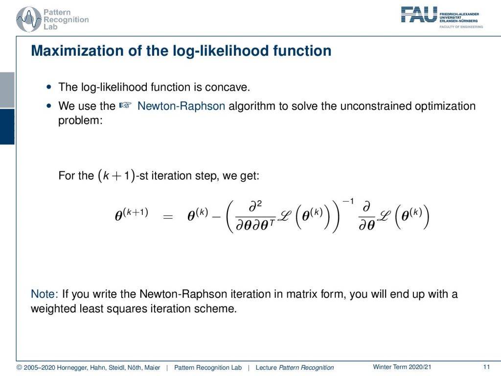
So, this is our maximization of the log-likelihood function. We’ve seen that it is concave meaning that the negative of the log-likelihood function is convex. This is the reason why we’re able to use the Newton-Raphson algorithm to solve this unconstrained optimization problem. If you want to apply this algorithm then you can see that we can get parameter updates simply by starting with a certain initial configuration for θ. Then we do updates on θ, so let’s say this we are in iteration k. Then we get the updated version θ^k+1 by computing the inverse of the Hessian matrix of our log-likelihood function times the gradient of the log-likelihood function with respect to our parameter vector θ. So, you can also write this up in matrix form. Then you essentially end up with a weighted least squares iteration scheme. Now the question is how do we come up with such a solution scheme and how do we actually determine this hessian and the gradient of the likelihood function. 

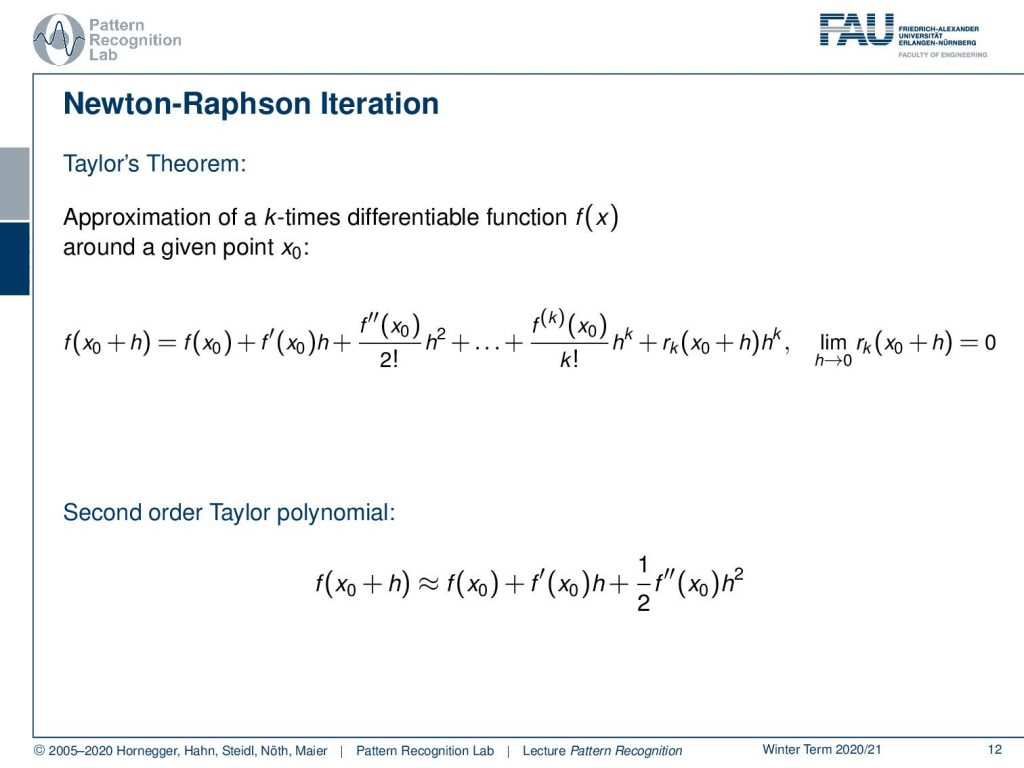
Now let’s start discussing the Newton-Raphson iteration. This is essentially motivated by Taylor’s theorem and it’s as you all know a way of approximating a k-times differentiable function f(x). If you have some initial point x₀ then the Taylor approximation tells us that we can essentially approximate this as f(x₀+h) is equal to f(x₀) plus the first derivative of x₀ times h plus the second derivative of the function at the position x₀ times h to the power of 2 divided of the factorial of 2. You can see that we essentially can go on with this until we have the complete Taylor series, which then goes all the way to k. If we compute the limit of h going to zero you see that this is going to be exactly zero so the error term that remains will also go towards zero. So, the closer we go to the initial position the closer our approximation will be. We can now use this in order to find an optimization strategy in particular we want to look into the second-order polynomial. In the second-order polynomial there we stop the expansion of the two terms. So, we have f(x₀) plus f ‘(x₀) times h, plus 1 over 2 times the second derivative of f(x₀) times h square. Now we’re actually interested in finding h. So, we can look at this approximation and compute the derivative with respect to h. If we do so you see that the first term cancels out and we can now see that also the h will go away and the h square will essentially be converted to h. 

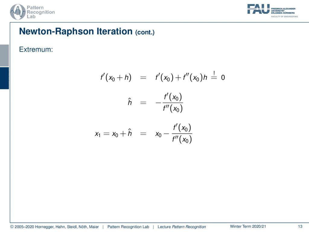
Exactly this is what we find on the next slide. So, this is the derivative of f and you can express this as the derivative of f at the position x₀ plus the second-order derivative of the function at the position x₀ times h. Now we want to find the minimum of this in order to solve for our strategy. So, we have to set this to zero. Now if you want to set this to zero you can see we can rearrange by subtracting f prime on the left-hand side which brings us to the right-hand side with a negative sign. We divide by the second-order derivative and this gives us an estimation of our ĥ. now we can reuse ĥ and find our x1., Sone so our updated scheme and this is going to be then simply x₀plus ĥ. This can be then written out as x₀ minus the first derivative of the function at x_0, divided by the second-order derivative of the function at x_0. Now if you bring this to a matrix notation you would see that the right-hand term can also then be rewritten as the hessian inverse times the gradient of the function. So, this is exactly our Newton-Raphson iteration. 

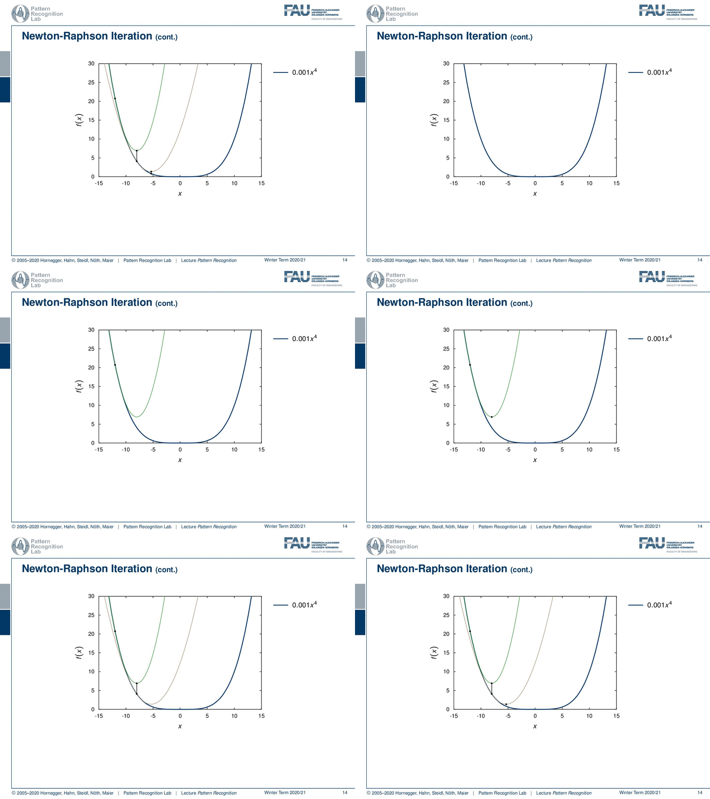
Let’s look at some examples where we show how this works. So, we need to initialize at some point. So, let’s pick this point for the initialization. Then we can set up our quadratic kind of solution scheme and the quadratic solution scheme will return this function. Now we determine our ĥ and ĥis going to be exactly here. So, this is our new update. Then we project this onto the original function. You can see then in the next step we can again produce this fit again determine our h head and this then will slowly bring us to the minimum of the function. You can see although we are only taking a second-order approximation, we will also converge towards a minimum in a function that is constructed by x to the power of four. Okay, so this is the scheme that we want to use to find our solutions. Now we still have to look into the different gradients and the hessian matrix of our problem.

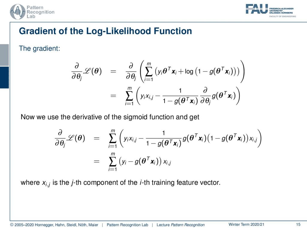
So, let’s recall our log-likelihood function and now we want to compute the derivative of the log-likelihood function with respect to our parameter vector θ. You can see here that we now have to solve this somehow. The nice thing is the derivative operator is linear. So we can essentially pull this in. Then you can see that the first term in the sum is actually linear and θ, so θ cancels out. So, it’s going to be only our y_i times x_i,j where x_i,j  is the respective component-wise formulation of the respective vector. Then also we need the derivative of the logarithm of the sigmoid function that we can essentially find in the following way. So, we need to use the chain rule of the logarithm which gives us the fraction here. Then we still need the derivative of the sigmoid function with respect to θ and we can now use the property of our sigmoid function. You can see here that then we essentially get the term g(θ^T x_i) times 1 minus g(θ^T x_i) times x_i,j. This is essentially the result of the chain rule and the differentiation here. Now we see that we have this term here twice and one time directly in the denominator and one time in the numerator. So, this one minus g(θ^T x_i). So, this cancels out and this brings us then to the derivative of our log-likelihood function that is simply given as the sum over all our m samples. Then we simply have to take the y_i minus the logistic function times the x_i,j, and x_i,j is the j-th component of the i-th training vector.

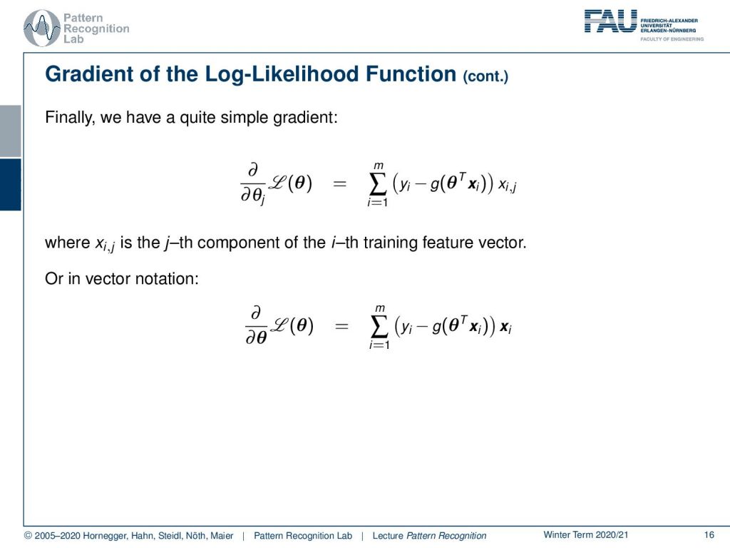
 So, this is already a quite simple gradient and we can furthermore slightly rearrange it a little bit and bring it back to vector notation. Here you then see that the gradient of the log-likelihood function with respect to θ can be expressed simply as the sum of the sigmoid function with the current parameter configuration and the sample and this is subtracted from the y_i and multiplied with the actual feature vector. Now we want to go ahead and also look into the hessian of this. So, we need to essentially derive this again with respect to θ to construct the second-order derivative of the log-likelihood function. Here you can see that we essentially then have to compute the derivative of the derivative and you see that we essentially have the sum again the derivative operator is linear. We see that we have the derivative with respect to θ. So, essentially our terms that involve the y_i and the x_i will cancel out. 

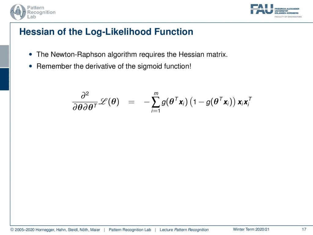
This then brings us to the second-order derivative or, hessian matrix. Here again, we have used the derivative of the sigmoid function we’ve seen that the y_i term essentially is canceling out because this was a constant term and it was not related to θ anymore. Then this essentially helps us to find the Hessian matrix here. So, this is also a rather straightforward formulation. So, you see that with the last couple of observations we were able to find an iteration scheme that was the Newton-Raphson iteration. In order to do that we need the gradient of the log-likelihood function and we need the hessian of the log-likelihood function. You’ve seen that we derived both of them in rather a couple of steps rather elegantly here in this set of slides. 

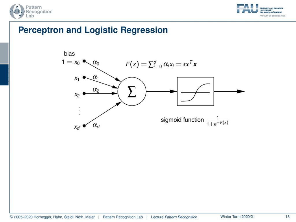
Note that there is also a relation to the perceptron. So, the perceptron is a very simple approach in order to create a trainable system. The perceptron is essentially a linear combination of some inputs and this is then mapped through a sigmoid function. So, you can see here that if I were to choose the perceptron in a high dimensional space, so I’m using the trick again to mapping to a more high dimensional space, then we can reuse the perceptron to find linear decision boundaries in this high dimensional space. So, everything that we discussed here can essentially be mapped into a perceptron with a sigmoid activation function. 

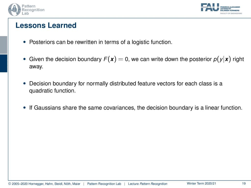
So, here’s some lessons that we have learned so far. We’ve seen that the posteriors can be rewritten in terms of a logistic function. Then we have seen that the decision boundary F(x) equals 0 is essentially related to the posterior right away. So, we can map the two together by using the logistic function. So, essentially if we know the decision boundary then we can immediately also derive the posterior probability. Also, the decision boundary for normally distributed feature vectors for each class is always a quadratic function. In the special case where we have the same covariances then the decision boundary is even a linear function. So, we’ve also seen that in the last couple of videos. So, this is also a very useful property.

So, next time we want to talk about a very simple approach, how to build a classification system. It is called the Naive Bayes classifier and we will have a short introduction to this idea. We will see that this naive Bayes is actually a very efficient way of finding classification rules very quickly and very efficiently. although it’s a very coarse approximation. 

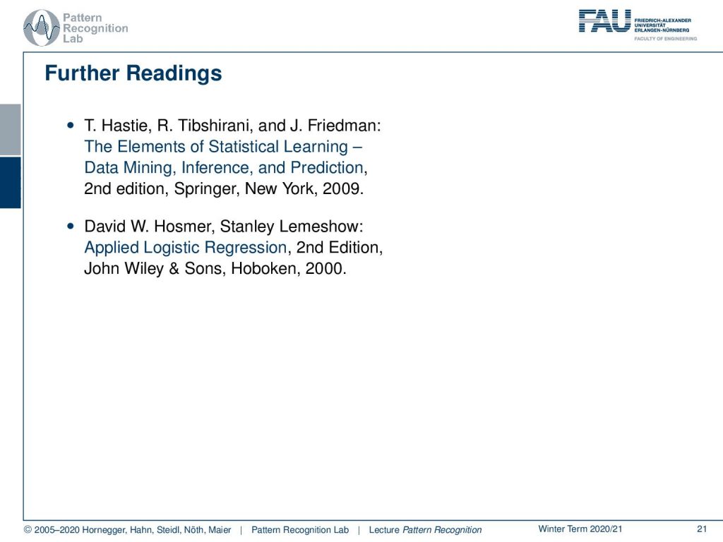
So, I also have some further reading for you again. I can only recommend “The Elements of Statistical Learning” here. This is really a great book and if you want to know more about logistic regression there’s also this wonderful book “Applied Logistic Regression”. 

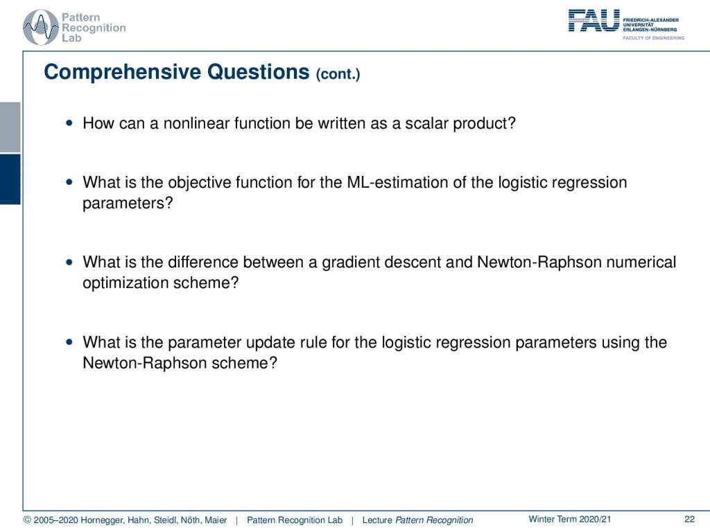
I also do have a couple of comprehensive questions that you will very likely find useful when you want to prepare for the exam. So, these are typical questions that could be asked in an exam or things that you should be able to explain in an exam situation. So, thank you very much for listening, and looking forward to seeing you in the next video. Bye-bye!

If you liked this post, you can find more essays here, more educational material on Machine Learning here, or have a look at our Deep Learning Lecture. I would also appreciate a follow on YouTube, Twitter, Facebook, or LinkedIn in case you want to be informed about more essays, videos, and research in the future. This article is released under the Creative Commons 4.0 Attribution License and can be reprinted and modified if referenced. If you are interested in generating transcripts from video lectures try AutoBlog

References

1. Trevor Hastie, Robert Tibshirani, Jerome Friedman: The Elements of Statistical Learning – Data Mining, Inference, and Prediction, 2^nd edition, Springer, New York, 2009.
2. David W. Hosmer, Stanley Lemeshow: Applied Logistic Regression, 2nd Edition, John Wiley & Sons, Hoboken, 2000.

Kategorie: Lecture Notes in Pattern Recognition