
These are the lecture notes for FAU’s YouTube Lecture “Pattern Recognition“. This is a full transcript of the lecture video & matching slides. We hope, you enjoy this as much as the videos. Of course, this transcript was created with deep learning techniques largely automatically and only minor manual modifications were performed. Try it yourself! If you spot mistakes, please let us know!
Welcome back to pattern recognition! Today we want to look into a more simple classification method that is called the Naive Bayes classifier.
The Naive Bayes classifier takes quite a few simplifying assumptions. Still, it’s widely successfully used and it often also outperforms much more advanced classifiers. It can be appropriate in the presence of high dimensional features. So, if you have really high dimensions because of the curse of dimensionality and the sparsity of training observations, it may make sense to simplify your model with Naive Bayes. Sometimes it’s even called idiot space. So, let’s look into the problem that it tries to tackle.
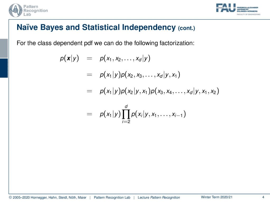
So, typically from the class-dependent probability density function, we can do the following factorization. You can see we have our observations x and if they are class-dependent and then we can rewrite the vector x in its components. So, we have the observations x1 to xd and they’re all given the class y. Now I can factorize this further which means that I can compute the class conditional probability for x1. Then I still need to multiply with the respected other probabilities and you can see that I can apply the same trick again. Then you can see that x2 is going to be dependent on y and x1 and we can write this up into the following product here. So, you see how we start building this on top and you see that we have all the different interdependencies. This is essentially nothing else than constructing a full covariance matrix here if you consider for example the Gaussian case.
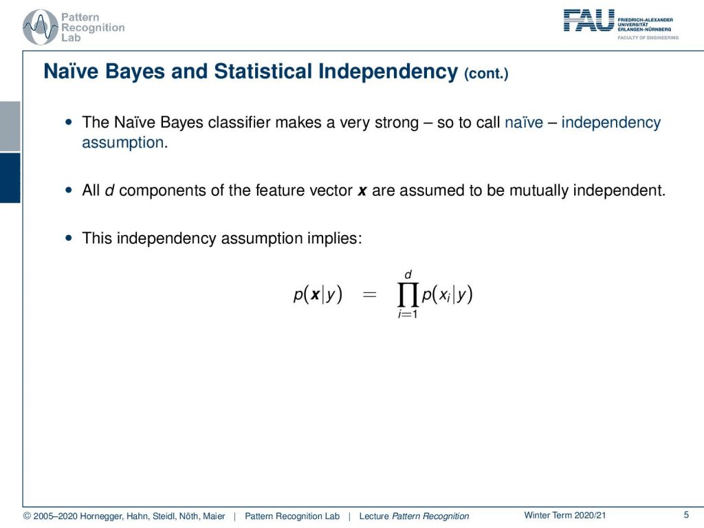
So, what do we do in Naive Bayes well Naive Bayes makes a very strong assumption. It assumes naively the independency of the dimensions. So, all d components of the feature vector x are assumed to be mutually independent. This then means that we can rewrite the actual class conditional probability for x as simply the product over the individual dimensions of x.
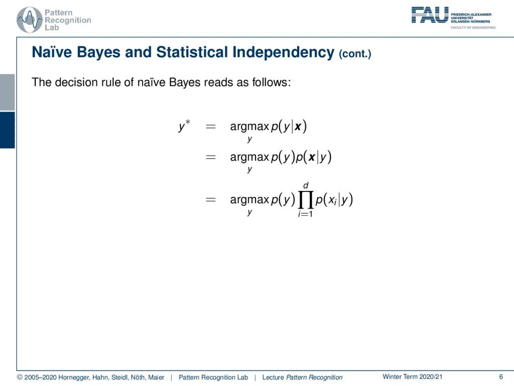
If we now apply this in the Bayes rule then you see that we still want to maximize our posterior probability with respect to y. Now we apply the Bayes rule. We’ve seen that we can get rid of the prior of x because in the maximization of y we are independent of x. So, this part is not considered here. Then we can see that we essentially can break this down to the prior of y times the component-wise class conditional probabilities. This is a fairly simple assumption and why would we want to do that.
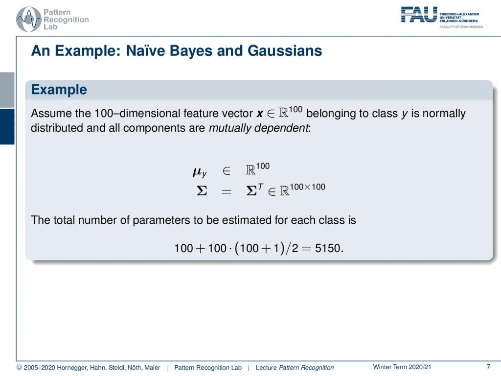
Well, let’s go back to our gaussian and if we now describe a 100-dimensional feature vector x that lives in a 100-dimensional space. Then if you belong to class y and this is normally distributed in all components that are mutually dependent you can see that we need a mean vector with a dimensionality of 100. We need a covariance matrix of dimensionality of 100 times 100. So this is fairly big. You can then even simplify this a little bit further because our covariance matrix actually doesn’t have complete degrees of freedom. But we actually have a triangular matrix because some of these components have to appear again. This means that we have essentially 100 unknowns in the mean vector and 100 times 100 plus 1 over 2 and this gives a total number of unknowns of 5150. Now let’s assume that they are mutually independent. This means that we still need to have a mean vector with 100 components. But we can break down our covariance matrix now. We see that we only have to estimate a single variance for every component of the vector. So, this is then a much simpler version and this brings us then down that we only have 100 plus 100 unknowns that need to be estimated. This reflects quite a bit of reduction in terms of parameters.
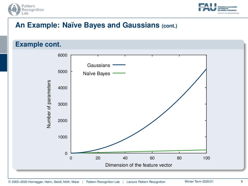
So, in this plot, we are actually showing the number of parameters on the y-axis and the dimension of the feature vector on the x-axis. You can see here that with Naive Bayes of course this is a linear relationship. While in a gaussian with full covariance we have something that is growing at a quadratic rate. Let’s look into the example and the effect of the modeling.
Here you see this example with two Gaussian distributions. They are both now using a full covariance matrix. If I break this down you can see here our decision boundary in black. Now if we use the naive Bayes it breaks down to the following decision boundary. So you can see it’s more coarse. It’s not such a great fit but it still does the trick. You can see as well that the estimated covariance parameters are also much simpler because it’s only two parameters per distribution.
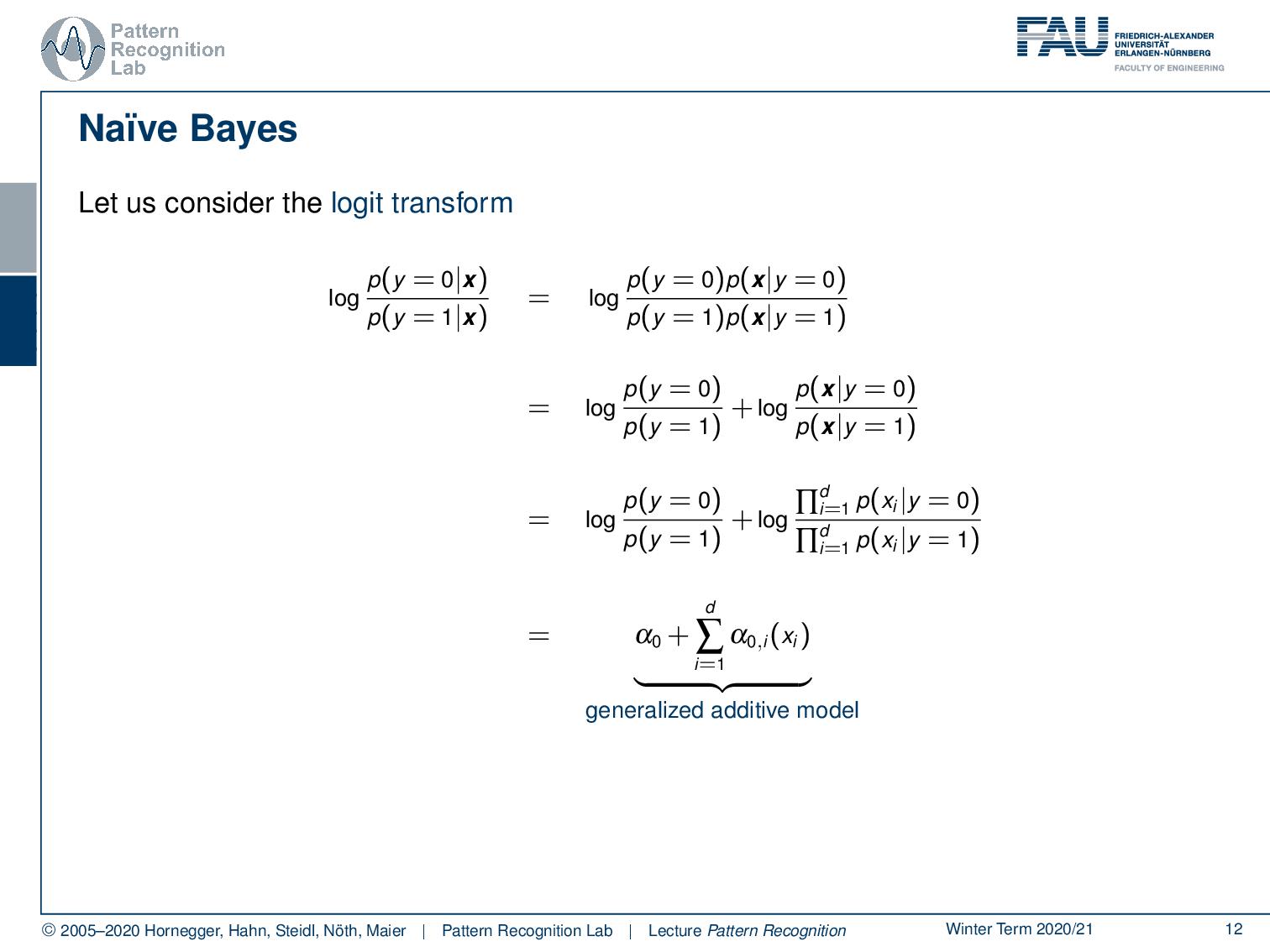
Also, we can consider the logit transform. So you remember if we want to look at the decision boundary then we take the posterior probabilities and divide them by each other and take the logarithm. We can of course reformulate this with the Bayes rule. This allows us then to split this fraction into two terms where we essentially have the prior on the left-hand side and the class conditionals on the right-hand side. Now we use this trick of Naive Bayes and we see that we can reformulate the class conditionals into products of the individual dimensions. This is a product that can be essentially used together with the logarithm. It can be converted into a sum. So, essentially you can see from this decision boundary here that we have something that is called a generalized additive model. So, we can formulate the decision boundary here in terms of this generalized additive model. This is essentially nothing else than the respective individual dimensions formulated in this sum here.
So, is there anything between Bayes and Naive Bayes? The answer is of course yes. There are multiple techniques that try to beat the curse of dimensionality. For example, you can reduce the parameter space as we did just with Naive Bayes. But of course, we don’t have to assume complete independence. So, we can maybe only use weak independence in contrast to complete mutual dependency or complete mutual independence. This is one thing that you can do and we will look into an example on the next slide actually. The other thing is of course parameter tying and this can both help you to reduce the dimensionality of the parameter space. Of course, there are also other approaches like the reduction of the dimensionality of the feature vectors. This brings us then to the domain of feature transforms.
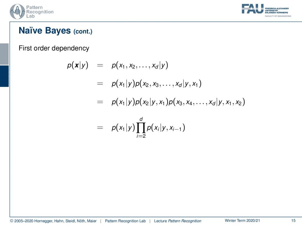
So let’s look at the ideas that we can do. So, you remember that we can write our class conditional probability in the following way. Now let’s introduce the first-order dependency. So, we start expanding here again and again and now we want to have a first-order dependency which that means that we can write this up as the product. Then we always have a dependency on the respective dimension and the neighboring dimension. So, it’s not completely dependent but only dependent on the neighboring dimension. If we apply this again then to a gaussian then you can see that we essentially come up with a covariance matrix that has this banded structure.
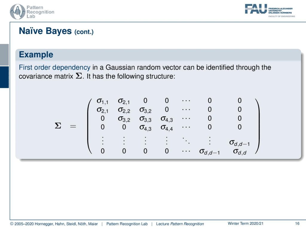
So, we have the diagonal as we would have in the Naive Bayes but we also have essentially one element of the diagonal that is also estimated. So, we have a slight kind of introduction of mutual dependence that we can model with this first-order dependency.
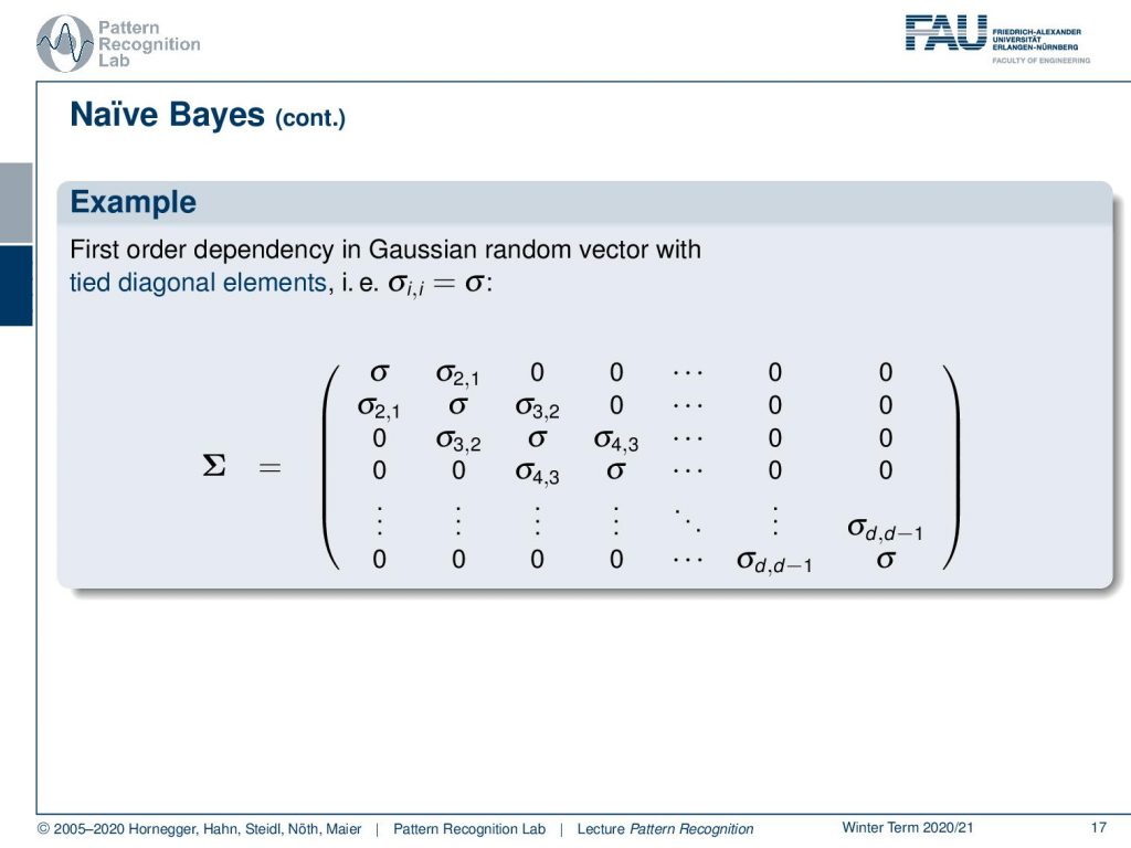
Another trick that we can use in order to reduce the parameters is to introduce tied parameters. Here for example we can say that all of the diagonal elements have to be the same parameter. Then we introduced just a single sigma on the complete diagonal. This would be one idea of parameter tying in order to further reduce the number of unknowns.
What are the lessons that we have learned here with Naive Bayes? Naive Bayes is rather successful so it’s being used quite a bit and it’s actually not such a bad idea. It does not require a huge set of training data because we have actually quite a few parameters and these fewer parameters can be estimated and also with fewer observations. Somehow we have to trade off the statistical dependency that we want to model in contrast to the dimensionality of the search space. So, if we do things like that then we can essentially trade the complexity of the model versus the actual number of observations. This is sometimes even a very good compromise and I can just tell you if you have few observations then you may want to give Naive Bayes actually a try.

Well in the next lecture we want to look into the other way of simplification and that is essentially dimensionality reduction. We want to look into something that is called discriminant analysis. The most popular one is the linear discriminant analysis and if you attended the introduction to pattern recognition you’ve already seen the linear discriminant analysis. We want to explore this idea a little bit further in the next couple of videos.
I do have a few further readings for you as well. So there’s of course “Pattern Recognition and Neural Networks where this topic is elaborated on. Also in Bishop’s book “Pattern Recognition and Machine Learning”, you can find further information about this topic.
Again I have a couple of comprehensive questions that may help you in preparation for the exam. This brings us to the end of today’s video. I hope you find this small excursion to the Naive Bayes classifier quite useful. You can see that we can use a couple of tricks by introducing independence in order to reduce the number of parameters and in order to simplify our estimation problems. Thank you very much for listening and looking forward to seeing you in the next video. Bye-bye!
If you liked this post, you can find more essays here, more educational material on Machine Learning here, or have a look at our Deep Learning Lecture. I would also appreciate a follow on YouTube, Twitter, Facebook, or LinkedIn in case you want to be informed about more essays, videos, and research in the future. This article is released under the Creative Commons 4.0 Attribution License and can be reprinted and modified if referenced. If you are interested in generating transcripts from video lectures try AutoBlog
References
- Brian D. Ripley: Pattern Recognition and Neural Networks, Cambridge University Press, Cambridge, 1996.
- Christopher M. Bishop: Pattern Recognition and Machine Learning, Springer, New York, 2006.