These are the lecture notes for FAU’s YouTube Lecture “Pattern Recognition“. This is a full transcript of the lecture video & matching slides. We hope, you enjoy this as much as the videos. Of course, this transcript was created with deep learning techniques largely automatically and only minor manual modifications were performed. Try it yourself! If you spot mistakes, please let us know!
Welcome everybody to Pattern Recognition. Today we want to talk a bit about feature transforms, and in particular, think about some ideas on how to incorporate class information into such a transform.
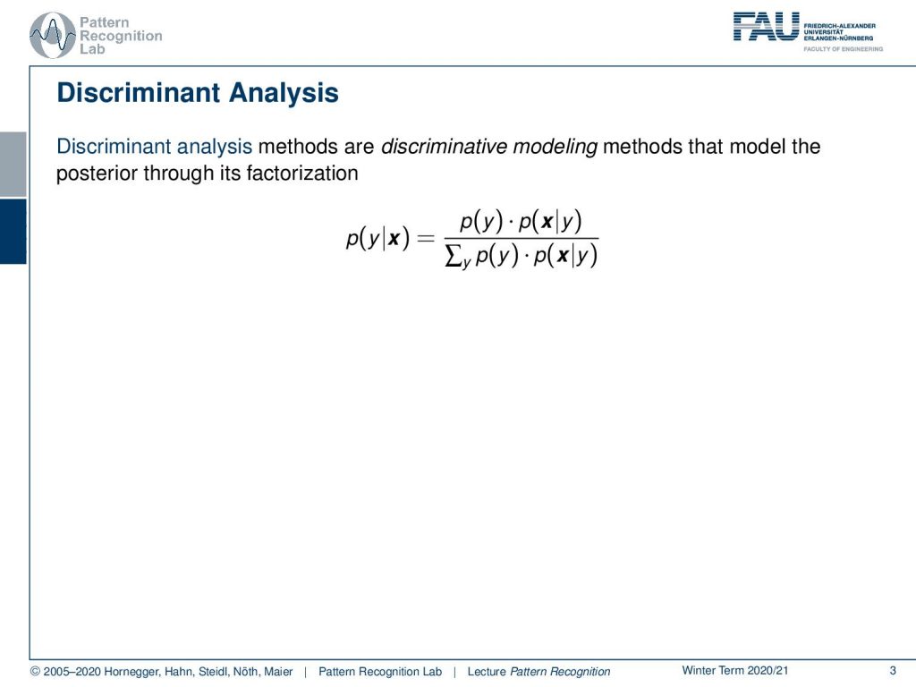
The path that we’re going towards is the discriminant analysis. This is essentially one way how we can think about using classes in feature transforms. So we will remember that if we do discriminate analysis, we do discriminative modeling. This means that we want to decompose the posterior in the factorization, where we use the class priors, and the class conditionals. So you see, using the base theorem and marginalization, we were able to decompose it into the following observations. Now, what we will do in the following is to choose a specific form of distribution for our probabilities.
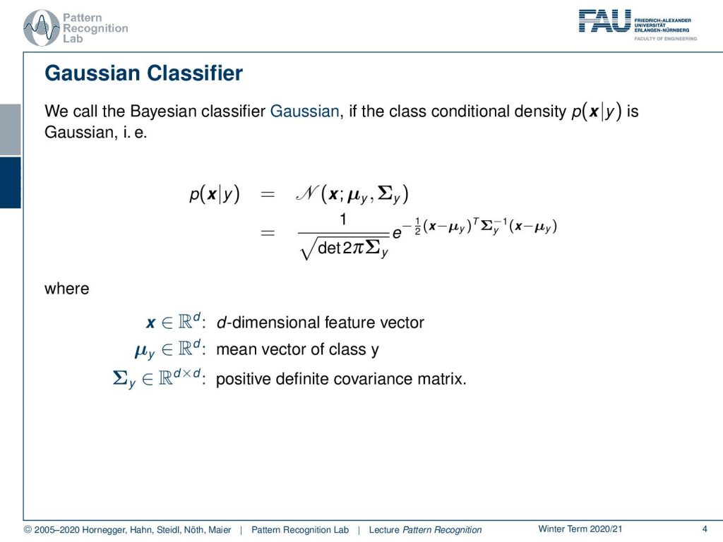
In particular, we want to use the Gaussian distribution for modeling our class conditionals. So, you remember that the Gaussian probability density function is given by a mean and a covariance matrix. Here we look into the class conditionals, which means that the means and the covariance matrices depend on the class y. This is why they have the respective index. And we remember that this is the formulation for the Gaussian probability. Of course, when you’re going to the exam, then everybody should be able to write this one down. You have the feature vector, the means for the class, and then also the covariance matrices, and they are positive definite. Please remember those properties.
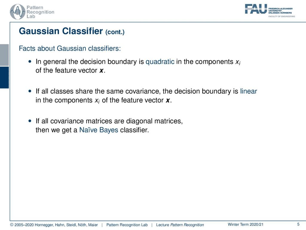
You also remember some of the facts about the Gaussian classifiers. If we try to model the decision boundary and everything is Gaussian, so the two classes that we’ve been considering are Gaussian, then we will have a quadratic decision boundary. If they share the same covariance, the decision boundary is going to be linear in the components of xᵢ of the feature vector. Also, we have seen the Naive Bayes approach. And the Naive Bayes, mapped onto a Gaussian classifier, will essentially result in diagonal covariance matrices.
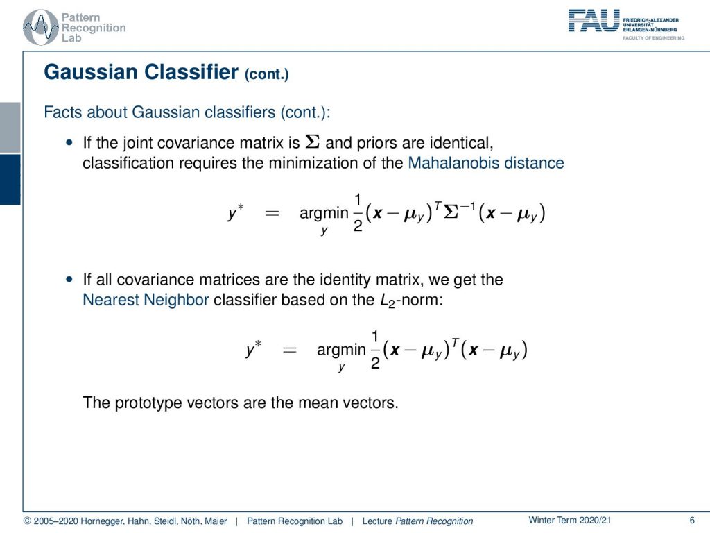
Also, if we would only have a single covariance matrix for all the classes and if the priors are identical, then the classification is essentially just a minimization of the so-called Mahalanobis distance. This is essentially a distance where you measure the difference to the class centers, and you weigh the distance with respect to the inverse of the covariance matrix. Then, if we simplify this further and if we had an identity matrix for the covariance matrix, we would essentially just look for the nearest neighbor. So here, the classifier would then simply compute the distance to the class centers, and then select the class center or prototype vector for the class which has the lowest distance. This would be just simply an L₂ or Euclidean distance neighboring approach.
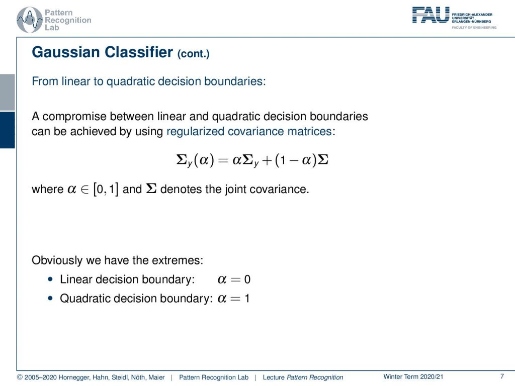
There are also ways how to somehow incorporate a little bit of additional information in the covariance matrices. We can essentially switch from linear to quadratic decision boundaries by mixing the modeling approach. So you could model the total covariance here in Σ or you could have the class-wise covariance the distance Σᵧ. And we could introduce a mixing factor α that is essentially given between 0 and 1. This would allow us to switch between class-wise modeling and global modeling. So if we have α=0 we would end up with the global modeling, and this would yield a linear decision boundary. And if we choose α to be one, then we would get the quadratic decision boundary. So we can essentially start mixing the two.
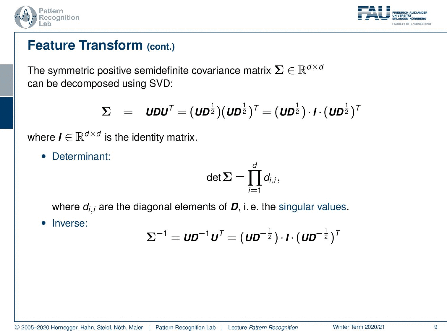
Now let’s think about the implications of feature transforms. The question that we want to ask today is: can we find a feature transform that generates feature vectors, so a transform of our vectors x? And this transform we want to call Φ, that shares the same covariance matrix. So can we do that? Well, let’s think a bit about the covariance matrix. There is a very useful tool that we can apply on all matrices that is the singular value decomposition. If you don’t know the singular value decomposition, I would recommend having a look at a refresher. There are quite a few things that we will now use in the following, properties of the singular value decomposition, that are extremely handy and we use it in Pattern Recognition all the time. So, please have a look at a refresher on singular value decomposition if you have trouble following the next couple of slides. The singular value decomposition allows us to decompose any kind of matrix into three matrices. This is typically then given as some U, D, and Vᵀ for a general matrix. Now that our matrix here is symmetric and positive semi-definite, then we can see that we essentially don’t need the V, but we just have U again. And we have the decomposition U D Uᵀ. U is an orthonormal matrix, so you can essentially interpret it as a rotation matrix. D is a diagonal matrix that has the singular values on the diagonal. This decomposition is possible for any kind of covariance matrix. Now we know that D is a diagonal matrix, so we can split D up and we take the square root on the diagonal elements. This gives us then D to the power of 0.5, so 1 over 2. So, we apply square roots on the diagonal, and then we can essentially split D up. And we see that we have two times the same expression, so U times D square root times U times D square root transpose. And if we already have this configuration, then we can also easily add an identity matrix in the center. This is simply the matrix that is diagonal and just has ones on the diagonal elements. It doesn’t change anything in terms of matrix multiplication, so we can simply add it here. If we analyze this term, then we can also see that we can get the determinant very easily because the determinant of our covariance matrix is then simply the multiplication over all the diagonal elements in D. This is essentially a property of the singular values. Also, the inverse is quite easy to get in this case because we can apply the inverse to our matrix factorization, to the singular value decomposition. The nice thing is that U is simply an orthonormal matrix, which means that its inverse will be given by its transpose. So, we can find the expression as U times D inverse times Uᵀ. Now, D is again a diagonal matrix, so if we want to invert D, we simply take one over the diagonal elements. This is also fairly easy to do. And then we see that we can write up the inverse of the covariance matrix simply as U times D to the power of -0.5. Meaning that we take this 1 over the square root of the singular values here, times the identity matrix, and then again, the same term U D to the power of -0.5 transpose.
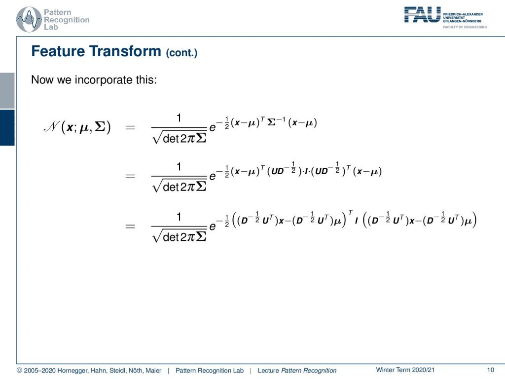
This is a quite useful decomposition because we can now apply it to a general Gaussian distribution. And if we apply it here to our Gaussian, then we have the original definition. We can now replace the covariance matrix here with the decomposition that we found earlier. And what you see here is that we essentially can model the covariance as this matrix product. And on the left-hand side and right-hand side we have essentially the same term. So, we can also move this term into the brackets regarding the actual observation x and the mean vector. This then brings us to the observation that we can essentially transform our distribution in a way that the actual covariance matrix becomes an identity matrix.
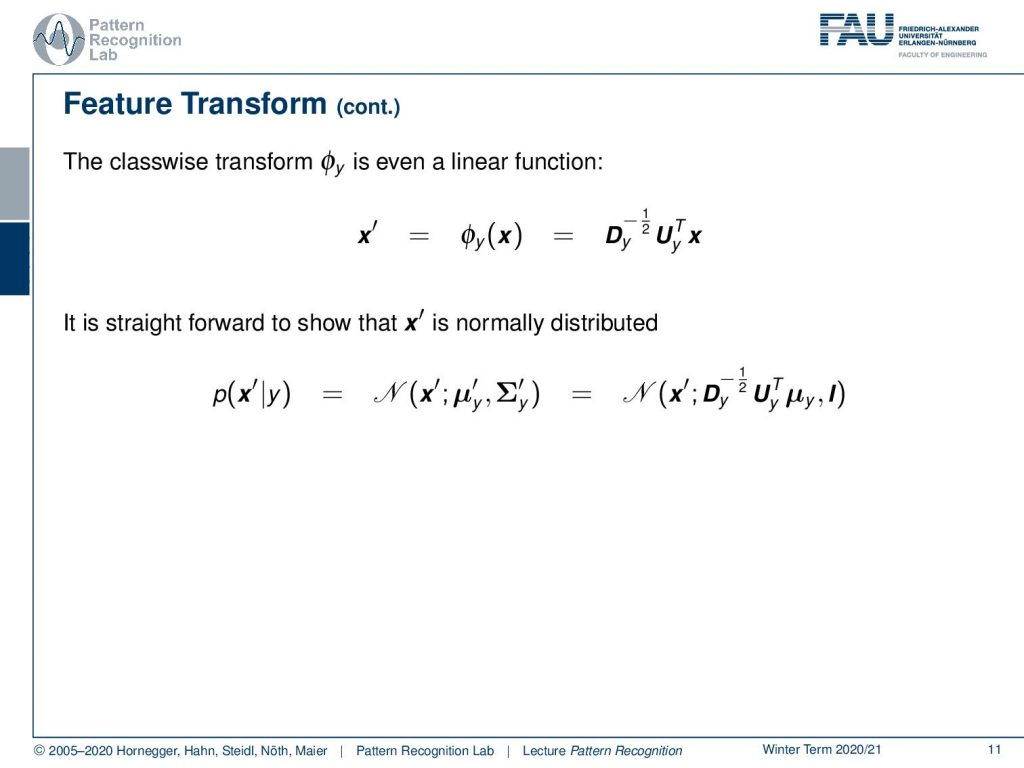
So, you see that we now take this out, and we again map into the class-wise feature space, so we have the Gaussian distribution for every class. Then we can essentially derive a feature transform for every class that incorporates essentially the decomposition of the respective covariance matrix of that class. This allows us to transform into a space that we here indicate as x′. This is a space in which all of the classes are mapped into a feature space where the Gaussian distribution has an identity matrix as covariance. So, how can we show that this is still a normal distribution? Well, we can simply plug in our feature transform on our x′ and use the definition. The x′ is simply a linear function on the input space. This means that we also have to transform the means. But we can then also see that the covariance matrix is mapped onto an identity matrix.
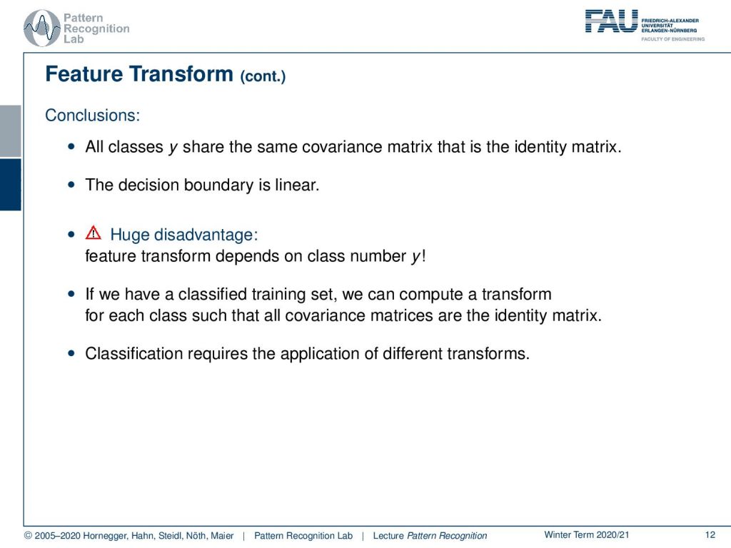
We can draw some conclusions. All of the classes y now share the same covariance, this is the identity matrix, and the decision boundary is linear. Note that this also has a huge disadvantage because the feature transform depends on the number of classes. So, we have a different feature transform for every class. And if we have, of course, a classified training set, we can compute this transform for each class such that the covariance is mapped onto the identity matrix. But if you want to apply this in a classification scenario, you would have to know to which class the respective sample belongs in order to apply this transform. This is kind of counter-intuitive because the class is actually the hidden information that we don’t have access to, so we can’t apply this concept straight forward in this way. But it already shows us some interesting ideas on how we could use essentially a class-dependent feature mapping to get better properties for the separation of our classes. This is kind of the first idea towards discriminant or linear discriminant analysis.
And this is then what we want to talk about next time. Next time, we want to look into how we can work with the particular version that we just derived, how to actually transform our features, and what kind of properties would then emerge in this feature space. I hope you liked this little video and I’m looking forward to seeing you in the next one! Bye-bye.
If you liked this post, you can find more essays here, more educational material on Machine Learning here, or have a look at our Deep Learning Lecture. I would also appreciate a follow on YouTube, Twitter, Facebook, or LinkedIn in case you want to be informed about more essays, videos, and research in the future. This article is released under the Creative Commons 4.0 Attribution License and can be reprinted and modified if referenced. If you are interested in generating transcripts from video lectures try AutoBlog.
References
Lloyd N. Trefethen, David Bau III: Numerical Linear Algebra, SIAM, Philadelphia, 1997.
Matrix Cookbook, https://www.math.uwaterloo.ca/~hwolkowi/matrixcookbook.pdf
T. Hastie, R. Tibshirani, and J. Friedman: The Elements of Statistical Learning – Data Mining, Inference, and Prediction. 2nd edition, Springer, New York, 2009.