These are the lecture notes for FAU’s YouTube Lecture “Pattern Recognition“. This is a full transcript of the lecture video & matching slides. We hope, you enjoy this as much as the videos. Of course, this transcript was created with deep learning techniques largely automatically and only minor manual modifications were performed. Try it yourself! If you spot mistakes, please let us know!
Welcome back to Pattern Recognition! Today we want to look a bit more into the logistic regression. In particular, we are interested in how to estimate the actual regression parameters, the decision boundaries.
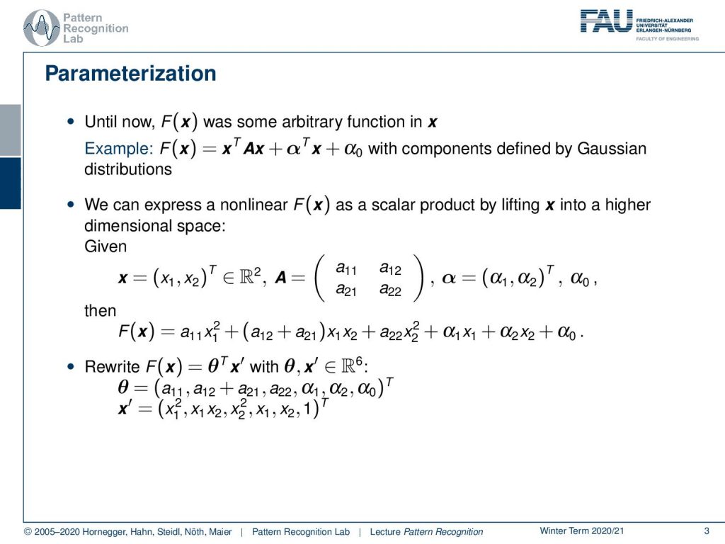
Today we look more into logistic regression. Until now we have seen that our f(x) was some arbitrary function. And we’ve seen, for example, that it could be formulated as a quadratic function, as we’ve seen with the Gaussian distributions.
So generally, we can express f(x) as a non-linear function. The idea that we want to use now is to linearize our estimation. What we will do is map our function into a higher dimensional space. So if you consider, for example, the quadratic function, we can see that we can express it component-wise in the following way. We know x is a vector consisting of x₁ and x₂. A can be written down in terms of the individual components and the same is also true for α. If you look for the component-wise notation, you see that f(x) can be written out in components. And we observe that the components we have in there are linear. So all the components of A and α are linear in this equation, and the x’s and so on appear in quadratic and linear terms. So this means that we can rewrite this into a function of x with some x′ where x′ is lifted to a six-dimensional space. So x′ is now rewritten from (x₁,x₂) to x₁², x₁ x₂, x₂², x₁, x₂, and 1. If we do that, then we can rewrite the entire equation into an inner product of our parameters. And the parameter vector is now a₁₁, a₁₂+a₂₁, a₂₂, α₁, α₂, and α₀. This is a kind of interesting observation because it allows us to bring our non-linear quadratic function into a linear combination that is linear in the parameters that we wish to estimate. This is a pretty cool observation because if we use this now, we can essentially map non-linear functions into a higher dimensionality. And in this higher dimensionality, we are still linear concerning the parameters.
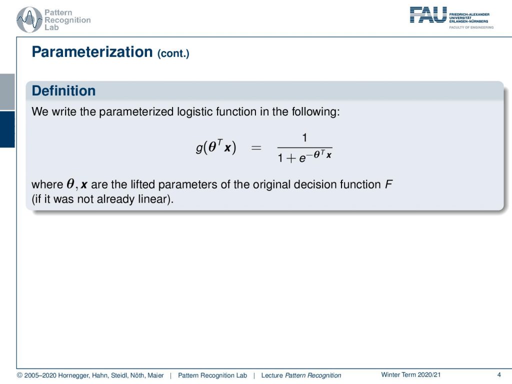
So, we can now remember our logistic function. We can see that if we use this trick, then we can essentially take our logistic function and apply it in this high-dimensional parameter space. So we don’t have to touch the logistic function. All that we have to do is to map essentially the axis into a higher dimensional space. But we can then use, instead of the version where we were using, the f (x). This could be a general non-linear function that we can replace now with our parameter vector θ. We essentially have the θ ᵀx, which is a linear decision boundary, but in a higher-dimensional space. And we can now use this and explore this idea a little further.
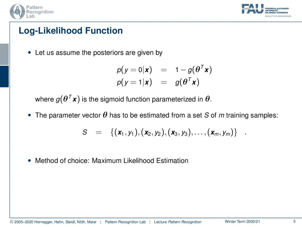
Also, we want to assume the posteriors to be given by two classes. We have the class y=0 and y=1. If we do so, we can write down the probabilities of the posteriors as 1-g(θ ᵀx ). g(θ ᵀx) is where we essentially reuse our logistic function or sigmoid function. And the thing we are interested in now is the parameter vector θ. So somehow, we have to estimate θ from a set of m training observations. And you remember, we are in the case of supervised learning here. So we have some set S, which is our training data set, and it contains m samples. There are essentially coupled observations where we have some (x₁, y₁) and more of these tuples up to m. Now the method of choice is the Maximum Likelihood Estimation. If we want to use that, then let’s look a bit into the formulation of how we want to write the posteriors.
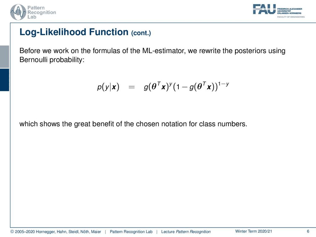
We can rewrite this as a Bernoulli probability. The probability of y given x can be rewritten using our logistic functions. So, now we use the logistic function to the power of y. If we are in the other case, then it’s going to be 1 minus the logistic function to the power of 1-y. You remember, we had our y essentially either 0 or 1. In this particular choice, we can now see that our probability, depending on which class we are having in the ground truth, will either choose the one or the other one. Because if you take something to the power of 0 then it will simply return 1 and the respective term will cancel out. So this kind of notation is very beneficial.
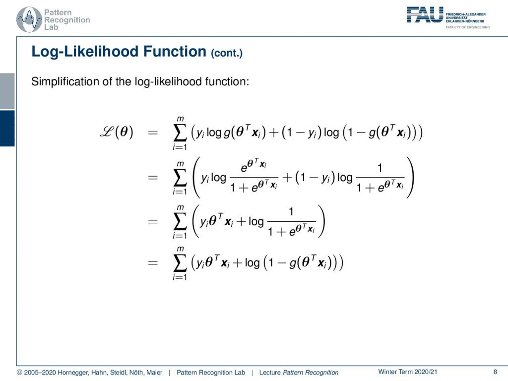
Now let’s go ahead and look into the log-likelihood function. We can write up the log-likelihood function as the logarithm of our general probability. We assume that all of the training samples are mutually independent. So we can simply then write this up as a product over all the posterior probabilities. This is kind of useful, because if we now apply the logarithm, then we see that the maximum of this function does not change, and still, we can reformulate it. Our product turns into a sum, and then we can also pull the logarithm inside, which is converting our product into the sum. Then we see it’s a sum over logarithms, and within the bracket, we see the definition of our posterior probability. This is, again, the formulation using the Bernoulli probability as mentioned previously. So here we have these terms with the logistic function. Now we can go ahead and use the property of the logarithm, where we then can pull the exponents in front of the logarithm. Then we get essentially the observation that in this line, all of the exponents have been moved in front of the logarithm. Also, we are breaking up the two terms of the sigmoid functions into a sum because they were a product. I can always convert a product within the logarithm as a sum of two logarithms as we did previously. This is already a first step towards simplifying this. But we can see that this can be simplified further. In the next step, we want to use the definition of the sigmoid or logistic function. You can see that the left-hand term we can essentially rewrite using the exponential function. And instead of using the notation with the negative sign, you can see that we already expanded the fraction on the left-hand side by adding the exponential term also to the numerator. This brings us then into a kind of notation that is very similar to what we see in the second term. There we have the logistic function in the formulation 1-g(θ ᵀxᵢ). This can also then be reformulated here on the right-hand side as 1 over 1 plus e to the power of θ inner product xᵢ. You see now why we did the adaption on the left-hand side, they both now have the same denominator. Now with this, we can simplify this further. You can see now that in the first term, we essentially see that we have e to the power of θ inner product xᵢ. If I apply the logarithm to this, then only yᵢ θ inner product xᵢ remains. On the right-hand side, then I still have some terms that I could not get rid of. But we still have the logistic function in there. But you can see that, if I look closely, we essentially have again the same formulation as previously. So we can move it back to the logistic function and we get the logarithm of 1 minus logistic function θ inner product xᵢ. This is already a simplification, and now you can see with this particular log-likelihood function I have two further observations that I want to hint you at.
What you can see here is essentially that the negative of the log-likelihood function will return the cross entropy of y and the logistic function of θ ᵀx. Also, note that the negative of the log-likelihood function here is a convex function. So this is a very nice property and we will use that in the following.

In the next video, we will talk about how to find the point of optimality and how to determine those parameters. So now we’ve seen the log-likelihood function, so we’ve seen which optimization problem we want to solve. This optimization problem will be solved in the next video. Thank you very much for listening and I’m looking forward to seeing you in the next video!
If you liked this post, you can find more essays here, more educational material on Machine Learning here, or have a look at our Deep Learning Lecture. I would also appreciate a follow on YouTube, Twitter, Facebook, or LinkedIn in case you want to be informed about more essays, videos, and research in the future. This article is released under the Creative Commons 4.0 Attribution License and can be reprinted and modified if referenced. If you are interested in generating transcripts from video lectures try AutoBlog.
References
T. Hastie, R. Tibshirani, and J. Friedman: The Elements of Statistical Learning – Data Mining, Inference, and Prediction, 2nd edition, Springer, New York, 2009.
David W. Hosmer, Stanley Lemeshow: Applied Logistic Regression, 2nd Edition, John Wiley & Sons, Hoboken, 2000.