Lecture Notes in Pattern Recognition: Episode 29 – Expectation-Maximization Introduction

These are the lecture notes for FAU’s YouTube Lecture “Pattern Recognition“. This is a full transcript of the lecture video & matching slides. We hope, you enjoy this as much as the videos. Of course, this transcript was created with deep learning techniques largely automatically and only minor manual modifications were performed. Try it yourself! If you spot mistakes, please let us know!

Welcome back everybody to pattern recognition. Today we want to look into a probabilistic estimation technique that allows us to estimate hidden information, the so-called expectation-maximization algorithm.

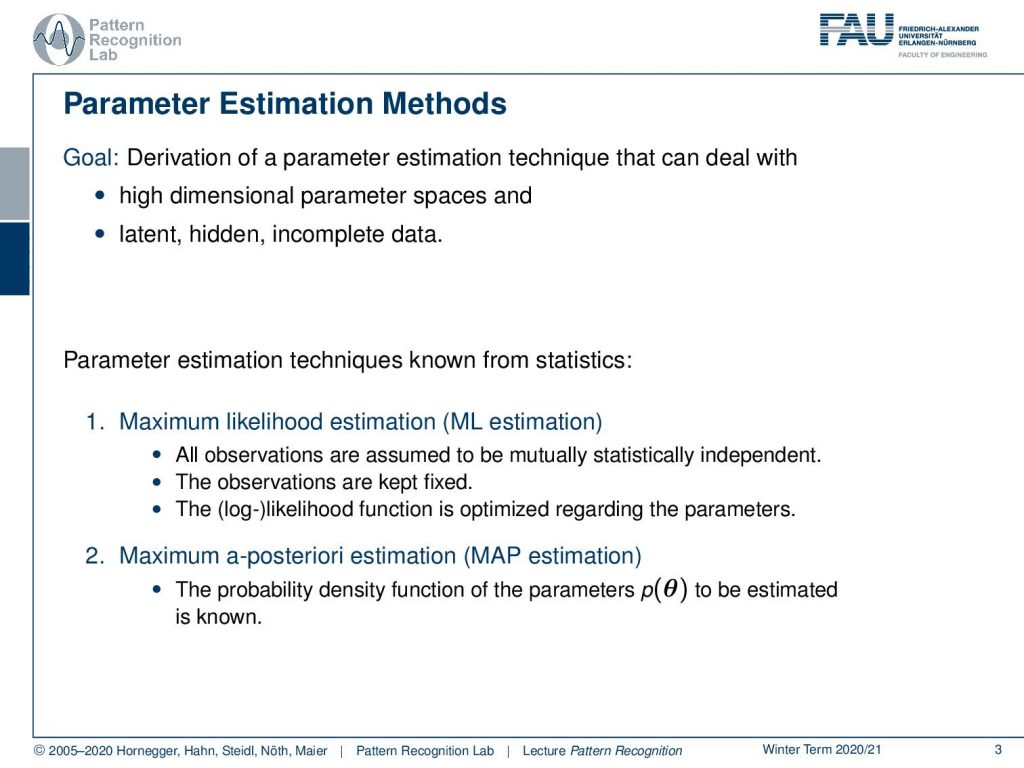
So let’s look into our slides so the topic today is the expectation-maximization algorithm and we want to use it for parameter estimation. So the goal is the derivation of a parameter estimation technique that will be able to deal with high dimensional parameter spaces, latent and hidden variables as well as incomplete data. So far we’ve seen the following techniques. We have seen the maximum likelihood estimation which is essentially assuming that all observations are mutually statistically independent. The observations are kept fixed and then the log-likelihood function is optimized with respect to the parameters. The other technique that we looked into was the maximum a posteriori estimation and there we essentially assume that there is a probability density function of our parameters. In order to do it of course we have to know how this function looks like in order to determine its parameters. 

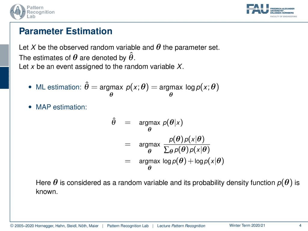
So generally we can now formulate this as X as an observed random variable and some parameter set θ. So the estimates of θ are denoted by θ̂ at and x can then be an event that is assigned to the random variable capital X. This gives us then the maximum likelihood estimation where we have the maximum over our likelihood function that then determines the optimal parameters θ̂. Typically we can write this up as a joint probability function. Now the other one is the maximum a posteriori estimation and here we determine our parameter θ̂ as the maximization over the probability of θ given some x and this can then rewritten by the Bayes rule and marginalization such that we then finally end up as the maximization of the logarithm of the prior θ plus the logarithm of x given θ. Now we essentially have a generative model where we know the distribution of x given θ and we are only interested in determining the optimal parameters. So θ is considered as a random variable and its probability density function is known.

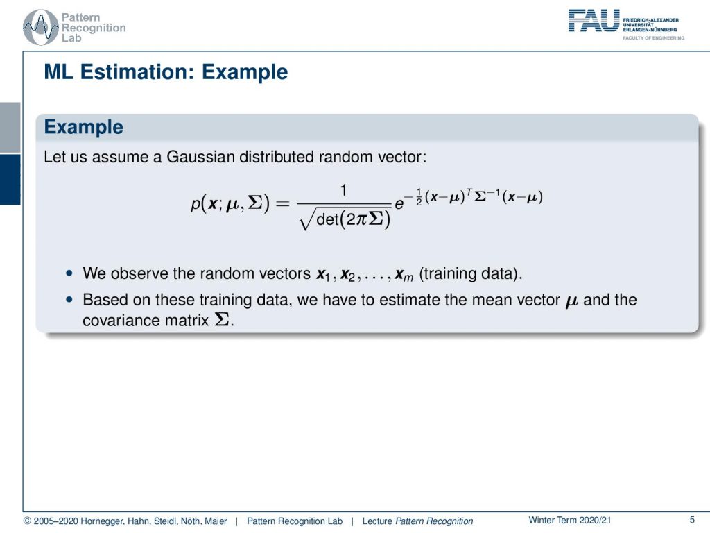
Let’s look into an example using maximum likelihood estimation. So here we assume a gaussian and you remember the gaussian and the normal distribution are of course very relevant also for the exam. So you see that we have this classical formulation as it popped out at various instances in our class and then we observe random vectors x₁ to x_m that form our training data. So based on these training data we now have to estimate the mean vector μ and the covariance matrix Σ.How can we do that?

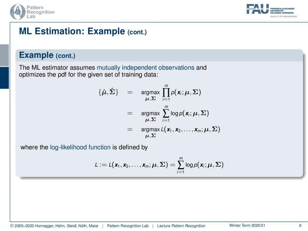
Well, we use the idea of maximum likelihood estimation and we assume that our samples are mutually independent which essentially allows us to write everything up as a large product. This large product is then maximized with respect to μ and Σ. We can essentially use the log-likelihood function and if we do so then we can even pull in the logarithm our product turns into a sum. This then allows us to essentially also write this up generally as the maximization of the log-likelihood function where we then have the observations as input and we seek to maximize it with respect to our μ and Σ. And here is our definition of the log-likelihood function that is simply the sum over the respective logarithmized probabilities.

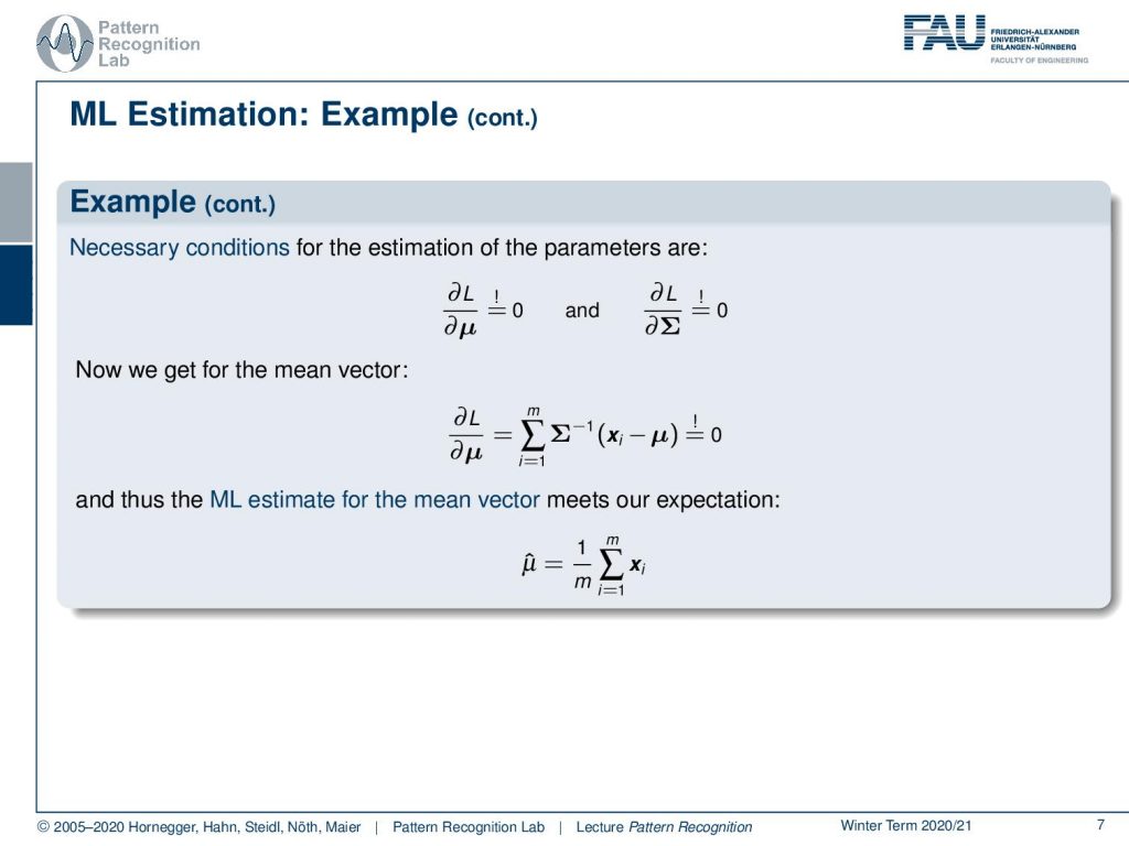
If you do so then you have to compute the partial derivative in order to compute the point of optimality and necessary conditions for these parameters are of course that the partial derivative with respect to μ equals to zero and the partial derivative with respect to Σ equals to zero. So we can actually do that, apply the definition of our gaussian and then we see that the prior term essentially can be removed because it’s not relevant for the optimization with respect to μ here. Then we essentially just remain with the exponent and this one we can then set to zero. Then we can also see if we solve the above equation then we essentially get the sum over all the observations divided by the number of observations as the mean vector. 

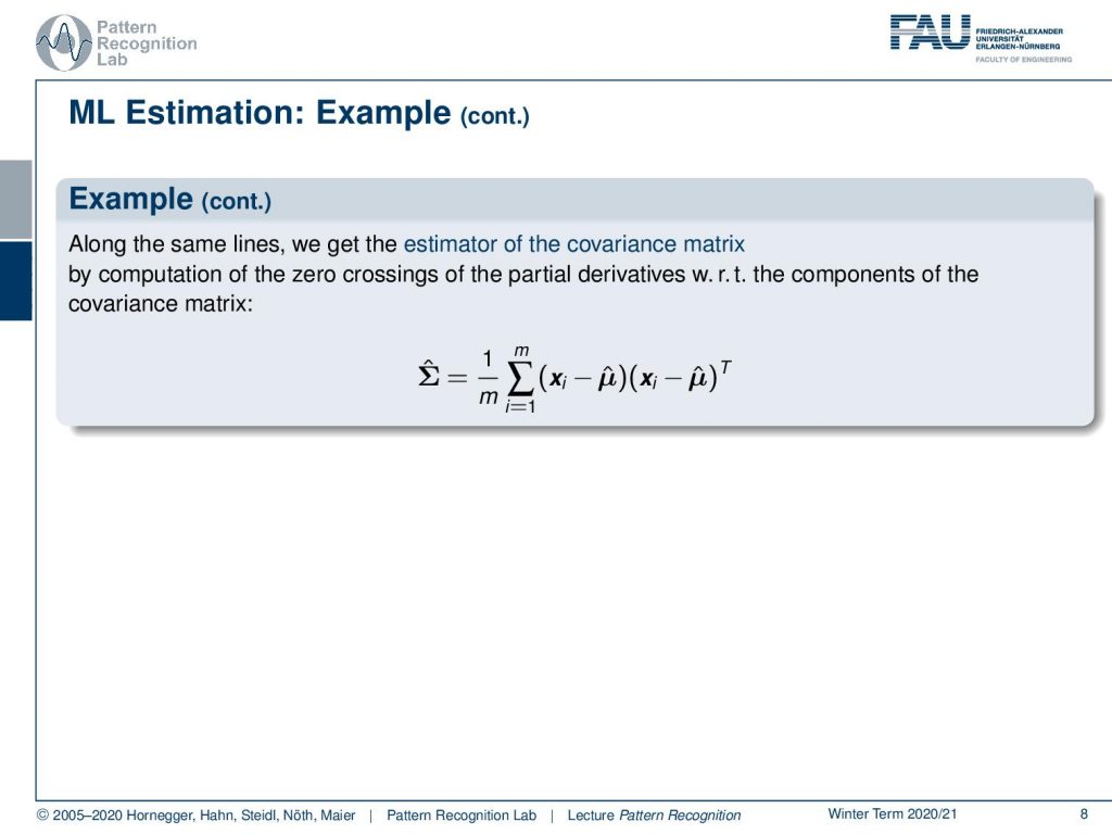
Now we can also estimate the covariance matrix and we do the same trick. We compute the partial derivative with respect to the log-likelihood function and then we determine its zero crossings. We can see that the covariance matrix then can be estimated as one over m where m is the number of training samples and then we have two vectors essentially and it’s actually twice the same vector it’s x_i minus μ̂ times x_i minus μ̂ transpose. So these are both column vectors so we essentially have degree one matrices and then a sum over all of the degree one matrices in our training samples that gives us then the estimate of the full covariance matrix.

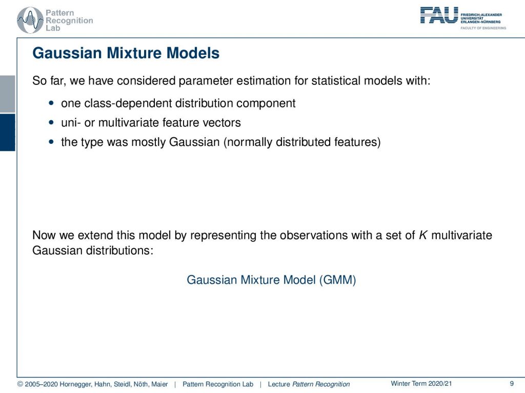
Now let’s go one step ahead and we want to consider so-called Gaussian mixture models. Because with the current Gaussians that we had so far we have quite a few limitations. So we had essentially one class dependent distribution component. We could have uni or multivariate features and the type was essentially mostly gaussian. So we had normally distributed features. Now we want to extend this and not just consider a single Gaussian distribution but we want to be able to model our probability density function as a set of capital K multivariate gaussian distributions. This gives rise to the gaussian mixture model. So a gaussian mixture model is able to describe any kind of superposition of different Gaussians. This is quite flexible because we can approximate arbitrary probability density functions using a superposition of Gaussians. So we essentially now go to the path that we want to describe complex probability density functions with an approximative technique where we use Gaussians as the basis.

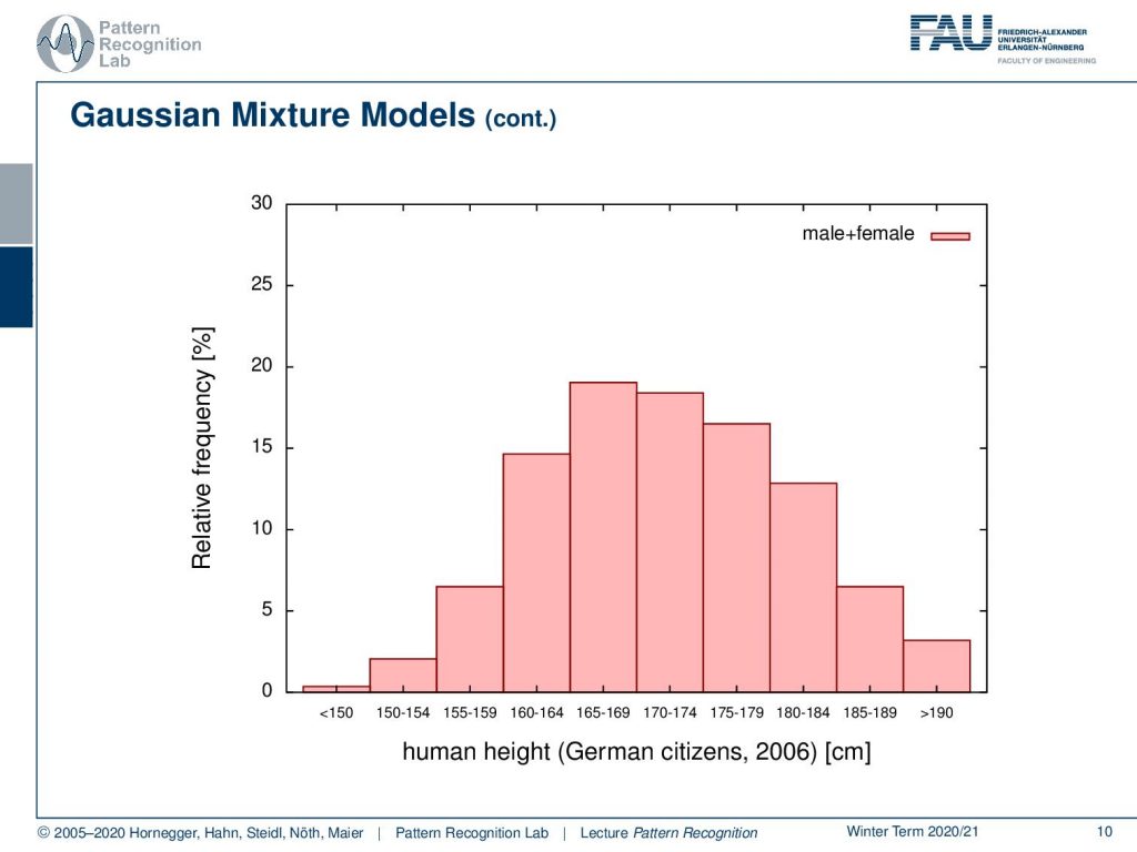
Let’s look into one example. So here we have a distribution and this is human height. This is for German citizens in 2006 and we show here the relative frequency and you see that we essentially have a distribution from somewhere below 150 centimeters up to above 190 centimeters. Now if you look closely at this distribution this is male plus female and now let’s look into the components.

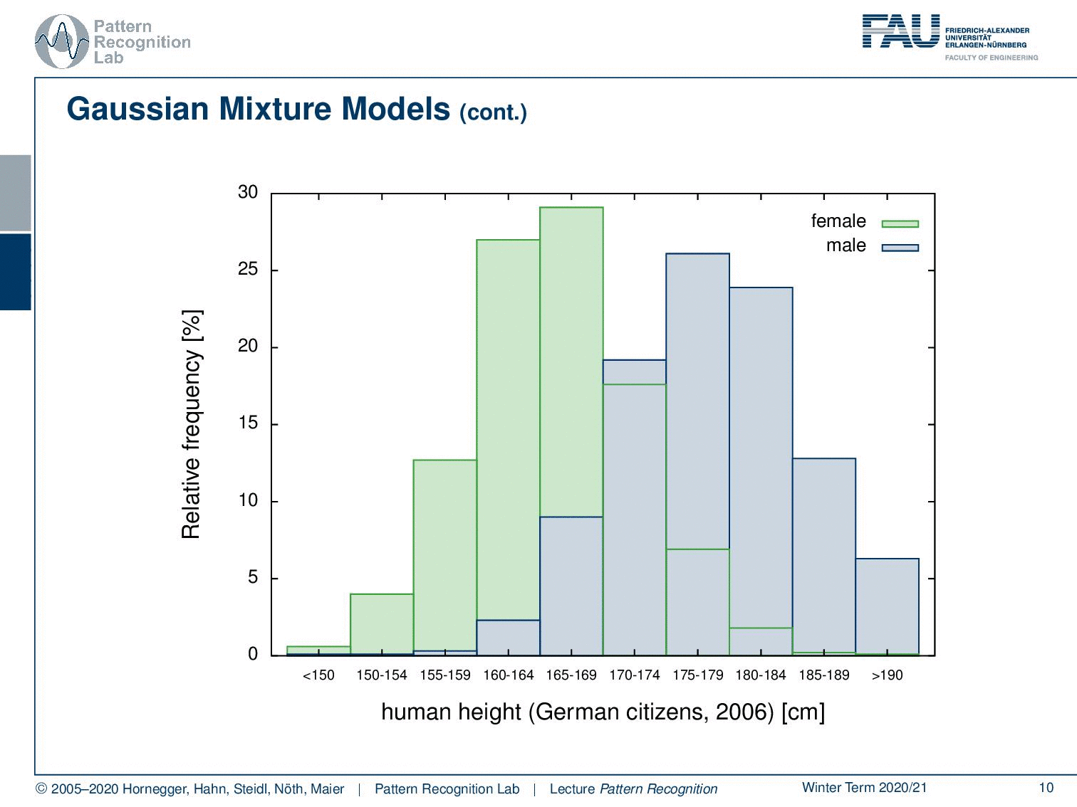
Here we have distribution for females and distribution for males. What you can see essentially is that the complete distribution is composed of parts. We actually observe the superposition of two Gaussians in this case.

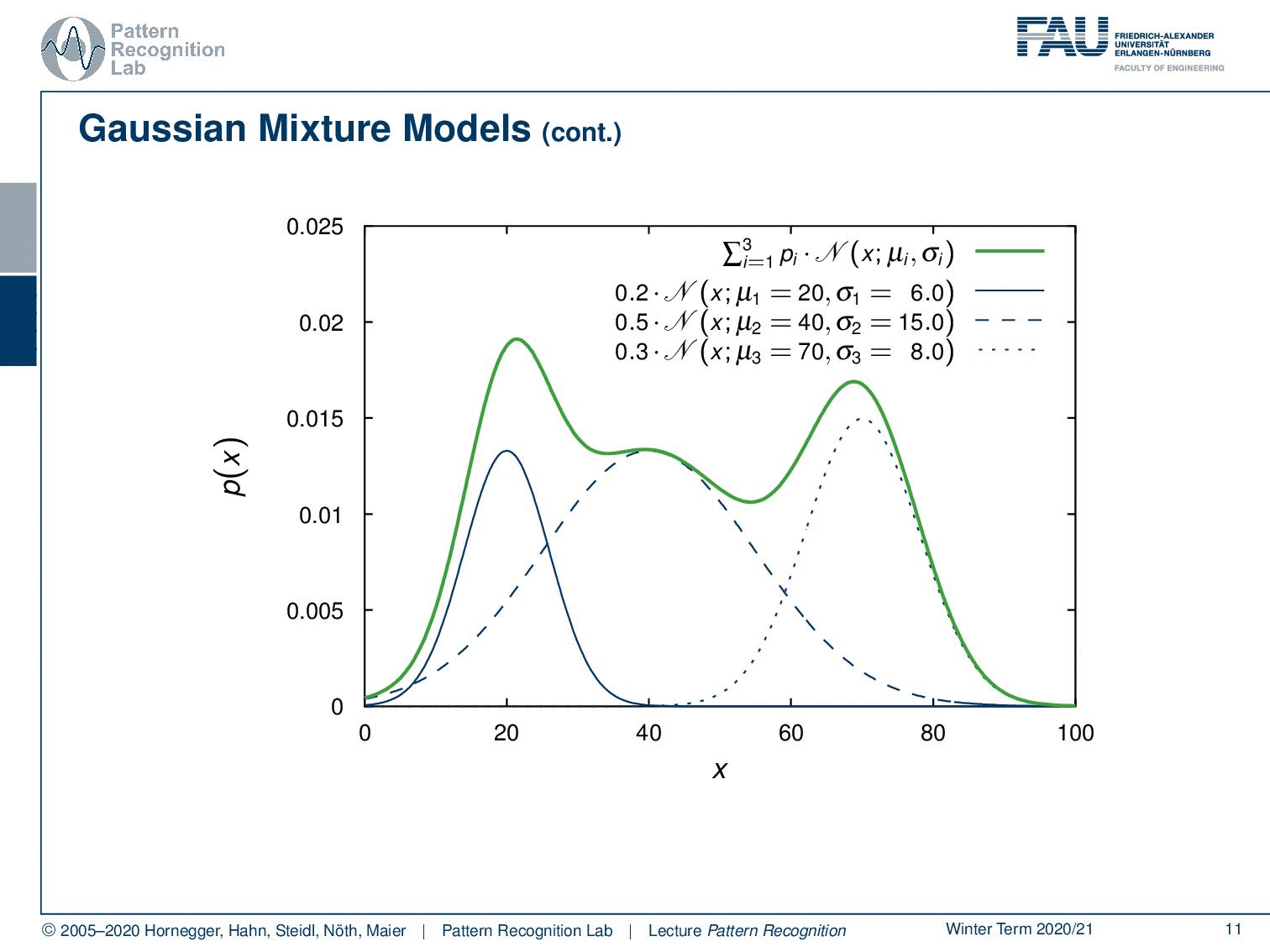
We could also have more Gaussians and you could even describe much more complicated probability density functions like the one that I’m showing here and this is actually the superposition of three Gaussians. So we have three gaussian components that have different priors. So not every component needs to be equally likely and this then allows us to mix the different Gaussians to approximate really complex probability density functions. Now we have the problem that we don’t need to estimate just a mean and a covariance matrix but the number of parameters increases. 

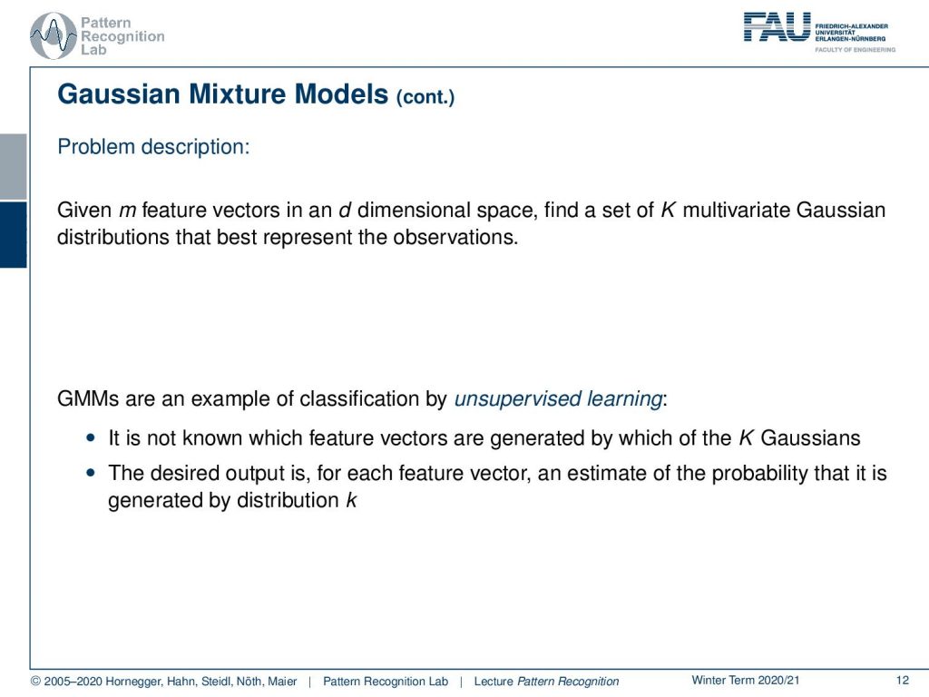
So generally we have given some m feature vectors in d-dimensional space and now the idea is that we want to find capital K multivariate gaussian distributions that represent best these observations. Now GMMs are an example of classification and we train using unsupervised learning. This means it is not known which feature vectors are generated by which of the K Gaussians. The desired output is for each feature vector an estimate of the probability that it is generated by the distribution k where k is the index of the capital K Gaussians.

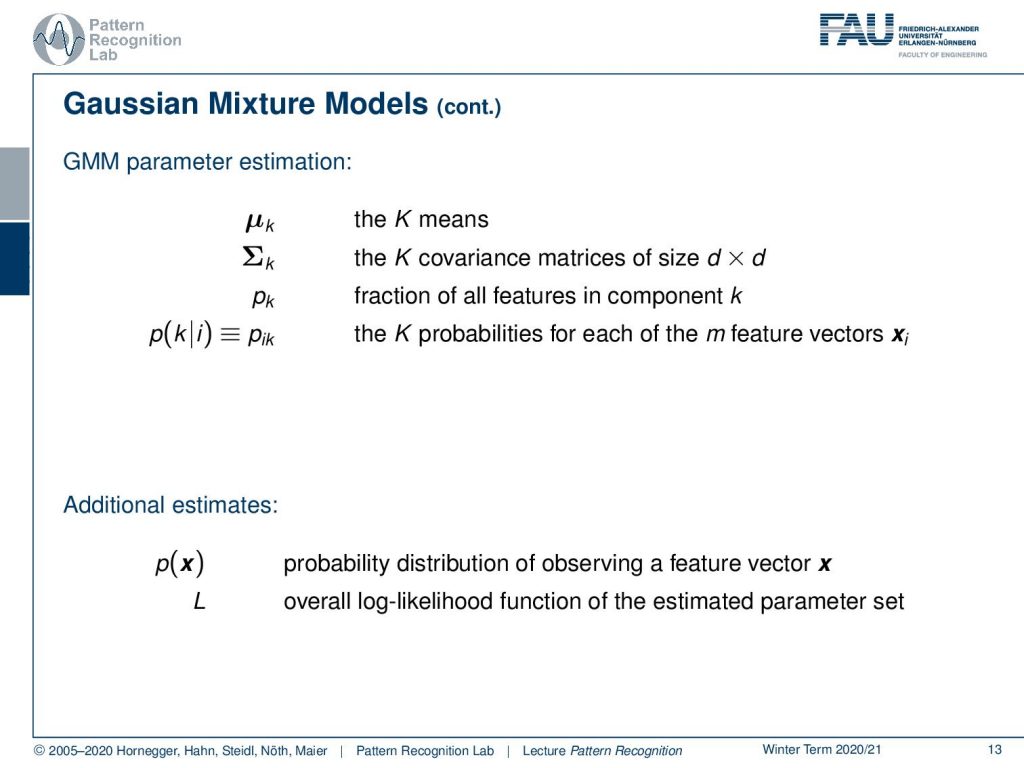
This then brings us to the following number of parameters. So we have generally for every one of the components k a mean and a covariance matrix. The mean has dimension d the covariance matrix has dimension d times d. Then we also have a fraction that is assigned to the respective component that describes how many of the observed training samples are actually associated with this component. We can further also define a probability that is p_ik or probability of component k given observation i that the probability of the respective feature vector is associated to this corresponding component. So for every feature vector, we observe capital K times this probability. Furthermore, we also have additional estimates that are the probability of the feature vector x that can then be described as a probability distribution of observing this particular feature vector. Then also the overall log-likelihood function of the estimated parameter set. 

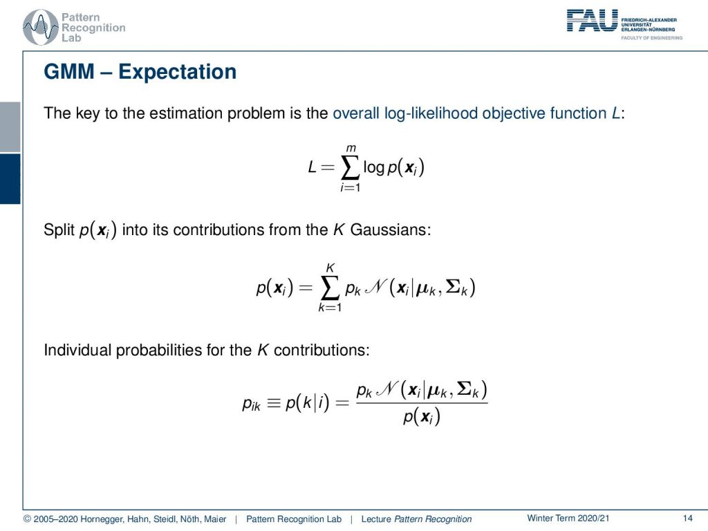
Now let’s look into our idea using the overall log-likelihood function. So we now know that our probability of x can be essentially described as a sum of capital K Gaussians. This then essentially means that we have to introduce the sum as the probability of x. Now we also want to introduce the individual probabilities for the k contributions and this is then our p_ik that we can write out as p_ktimes the Gaussian of the respective component divided by the probability of observing x.

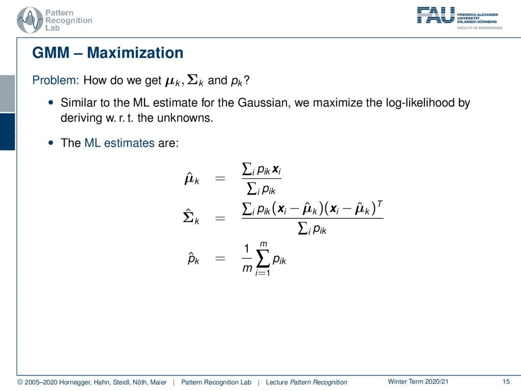
Okay so how do we get μ_k, Σ_k, and p_k. Well similar to the maximum likelihood estimate for the Gaussian we can maximize the log-likelihood by deriving it with respect to the unknowns. So we can do this and this will then yield to the following estimate. So we get a μ̂ for component k as the sum of the p_ik times the respective feature vector divided by the total sum of the p_ik. Also, we can determine in a similar fashion our estimate of the covariance matrix for k as well as the prior of this component. So you see that now we are able to describe the estimate but we essentially need this probability of the observation i to be related to the component k. Now, this is generally something that we can only observe if we would know already the parameters. So how can we guide this estimation process?

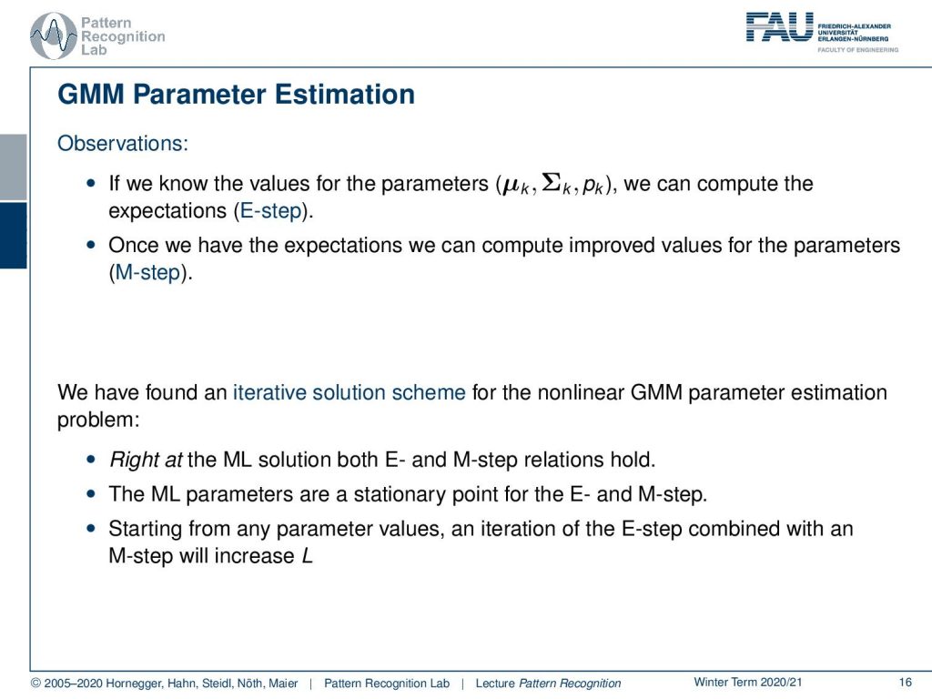
Now the idea is that if we know the values for the parameters then we would be able to compute the expectations. Once we have the expectations we could compute the improved values for the parameters in this so-called maximization step the M-step. So there’s the E-step and the M-step. So how do we do this? Well, this leads to an iterative solution scheme for the non-linear GMM parameter estimation and remember right at the Maximum Likelihood solution both the E-step and the M-step hold. So this means that the ML parameters are a stationary point for the E and the M step. Then starting from any parameter values and iteration of the E step combined with an estimation of the M step will increase the log-likelihood function. This then gives rise to an estimation algorithm and here we have the sketch of the EM algorithm for the GMM parameter estimation.

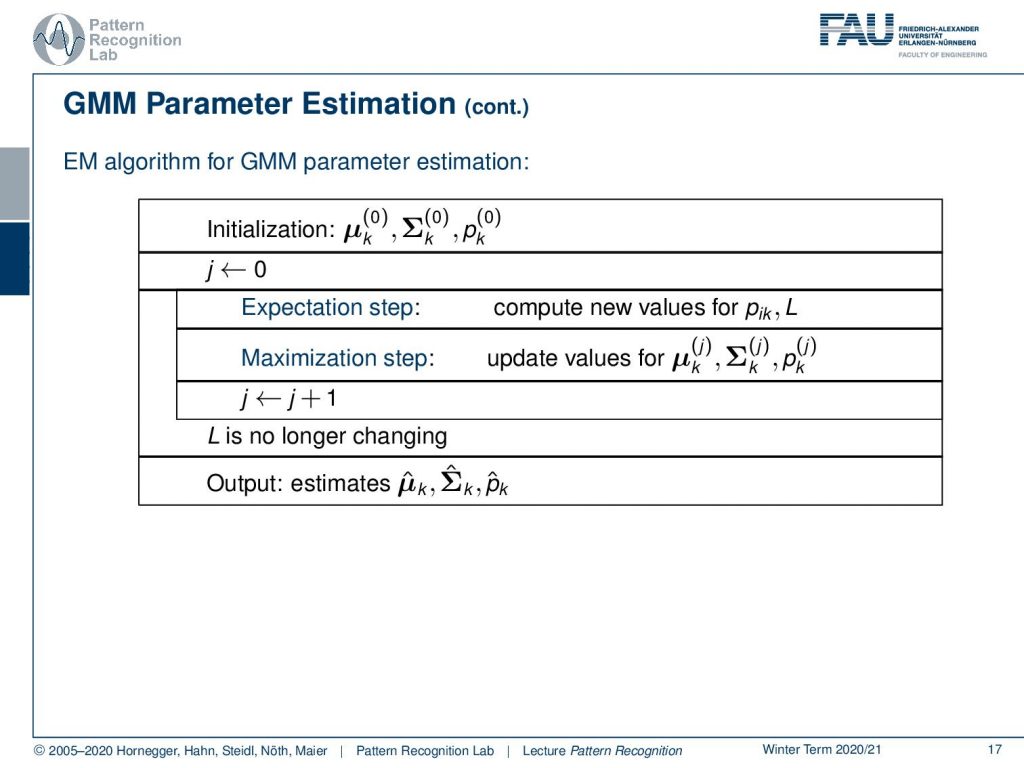
So you initialize with some μ_k some Σ_k and some p_k. Then you set the iteration counter to zero. You run the expectation step which means that you compute new values for p_ik and L and once you have computed those you can essentially run the maximization step which is then updating the values from μ_k, Σ_k, and p_k. Now we have those three values and they’re improved so we can increase the iteration counter and start iterating until our log-likelihood function is no longer changing. At this point, we have an optimal condition and we output the estimates μ̂_k, Σ̂_k, and p̂_khat. 

So this was the derivation for the GMM estimation obviously the expectation-maximization algorithm goes far beyond this and it can be applied on many many other occasions. This is why we look into the missing information principle in the next lecture and then we will look into a general solution scheme for EM type of problems. So thank you very much for listening and I hope you enjoyed this little video looking forward to seeing you in the next one. Bye-bye.

If you liked this post, you can find more essays here, more educational material on Machine Learning here, or have a look at our Deep Learning Lecture. I would also appreciate a follow on YouTube, Twitter, Facebook, or LinkedIn in case you want to be informed about more essays, videos, and research in the future. This article is released under the Creative Commons 4.0 Attribution License and can be reprinted and modified if referenced. If you are interested in generating transcripts from video lectures try AutoBlog

References

1. Easy to understand tutorial on ML estimation: In Jae Myung: ☞ Tutorial on maximum likelihood estimation, Journal of Mathematical Psychology, 47(1):90-100, 2003 
2. The classics for an introduction to the EM algorithm is: A. P. Dempster, N. M. Laird, D. B. Rubin: ☞ Maximum Likelihood Estimation from Incomplete Data via the EM Algorithm, Journal of the Royal Statistical Society, Series B, 39(1):1-38. 
3. W. H. Press, S. A. Teukolsky, W. T. Vetterling, B. P. Flannery: ☞ Numerical Recipes, 3rd Edition, Cambridge University Press, 2007.

Category: Lecture Notes in Pattern Recognition