Lecture Notes in Pattern Recognition: Episode 30 – Expectation Maximization Algorithm

These are the lecture notes for FAU’s YouTube Lecture “Pattern Recognition“. This is a full transcript of the lecture video & matching slides. We hope, you enjoy this as much as the videos. Of course, this transcript was created with deep learning techniques largely automatically and only minor manual modifications were performed. Try it yourself! If you spot mistakes, please let us know!

Welcome back to Pattern Recognition! Today we want to look a bit more into the EM algorithm. In particular, we want to learn how to apply it to other problems. We will start with the so-called missing information principle.

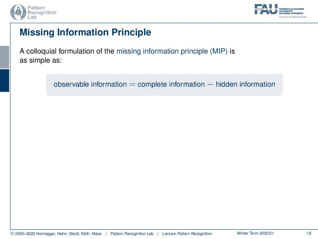
Now the missing information principle is as simple as that the observable information is given as the complete information minus the hidden information.

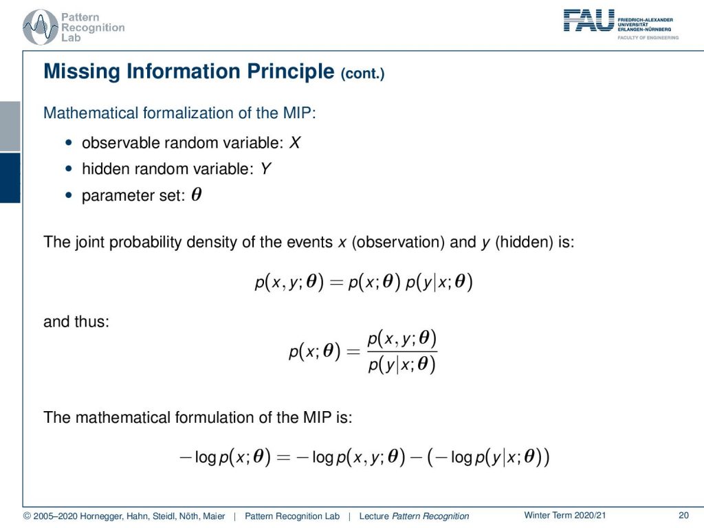
Now let’s look at this in a little more mathematical way. We can formalize the entire problem as the observable random variable X, the hidden random variable Y, and the parameter set θ. Now we can use this to formalize the joint probability density of the events x, the observable part, and the hidden part y as the probability of x and y, and parameter θ. This can be expressed as the probability of x;θ times the probability of y given x. Now we can reformulate this, and we see that our p(x θ) is given as the fraction of p(x,y;θ) divided by p(y|x;θ). Now we can look at this and apply the negative logarithm. So we can see that minus the logarithm of p(x; θ) is equal to minus the logarithm of p(x,y;θ) minus the negative logarithm of p(y|x;θ).

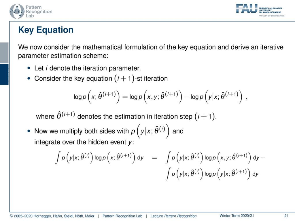
Now let’s rewrite this a little bit. The idea that we want to introduce is we want to write it in an iterative iteration scheme. Now we can write this essentially as the i+1 iteration and write this essentially in the same form, but with an additional iteration index. Now our θ is essentially the estimate of our parameter vector θ. So this is now indicating the parameter step. Now let’s multiply both sides with p(y|x) and the parameter vector in the eighth iteration, and we integrate over the entire hidden event y. So we introduce the integral and we multiply with this additional probability. Then this can be written as the integral on the left-hand side, and of course, also on the right-hand side, we can see that we can split the two integrals. We end up with something that is the probability of y given x and the parameter vector θ times above logarithms. And now you already see that this looks kind of familiar. So let’s look a little bit more on the left-hand side.

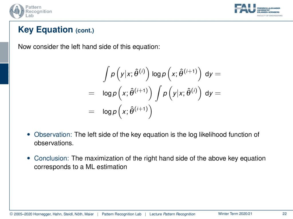
Here you can see that if we rearrange this a little bit, we can pull out the logarithm and the probability of x and θ⁽ⁱ⁺¹⁾. This then can be essentially rearranged as this logarithm, because the integral over p(y|x) over the entire domain of y is just going to be 1. So we remain with the logarithm of the probability of x. We can observe that the left-hand side of the equation is the log-likelihood function of our observations. We encountered this term previously and we can now use this to express the log-likelihood function. The maximization of the right-hand side of our key equation here corresponds to a maximum likelihood estimation.

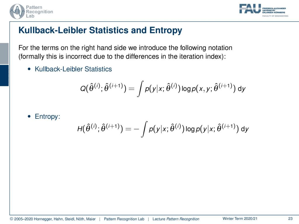
Now if we look at the terms on the right-hand side we see that we can introduce the following notation formally. This is a little bit incorrect, but it’s just a small alteration of the iteration indices. This then gives rise to the cobalt libra statistics that can be expressed as Q of the parameter vector θ  hat in iteration i. Iteration i+1 is given as the integral of p(y|x) times the logarithm of p of x and y and the integration over y. Furthermore, we observe the entropy, which is here defined as H between our parameter vector θ hat at iteration i and iteration i+1. This is the negative integral over the probability of y given x times the logarithm of the probability of y given x and the parameter vector in the next iteration.

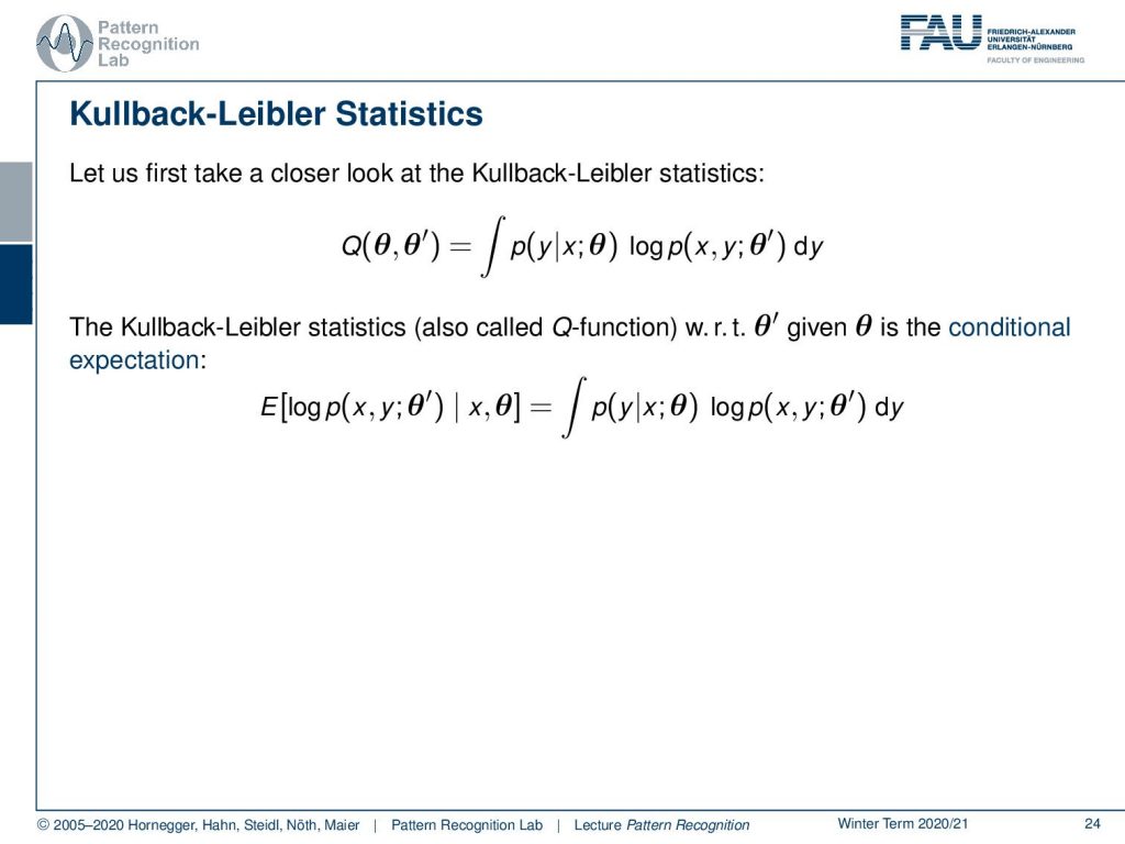
Now, let’s first have a closer look at the Kullback-Leibler statistics. If we look at the statistics between θ and θ′ and we write out the expression as an above equation, then we can see that the Kullback-Leibler statistics, which are also called Q-function concerning θ′ and θ, is nothing else than the conditional expectation of the log-likelihood of the joint probability of x and y.

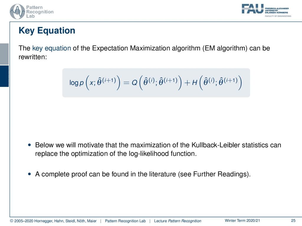
Now let’s have a look again at the key equation. You can see that we can now write it down as the log-likelihood function of x. This can be expressed as the Q-statistics plus the entropy of the old parameter set and the new parameter set. Now we want to motivate that the maximization of the Kullback-Leibler statistics can replace the optimization of the log-likelihood function. Note that we only look at this on a rather coarse level. A complete proof can be found in the literature if you have a look at the further readings.

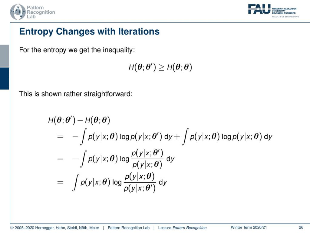
Let’s look a bit into the properties of the entropy. We get the following inequality for entropy, that if you have a parameter set θ and the parameter set θ′, then this entropy is generally larger than the entropy of the parameter set of itself. Now to show this is rather straightforward we can subtract the two terms from each other. Then we can plug in the definition of entropy. And now you can see that I can merge the two integrals by just converting the subtraction of two logarithms into a fraction. Furthermore, you can see that I can flip the sign by flipping the fraction inside the logarithm. 

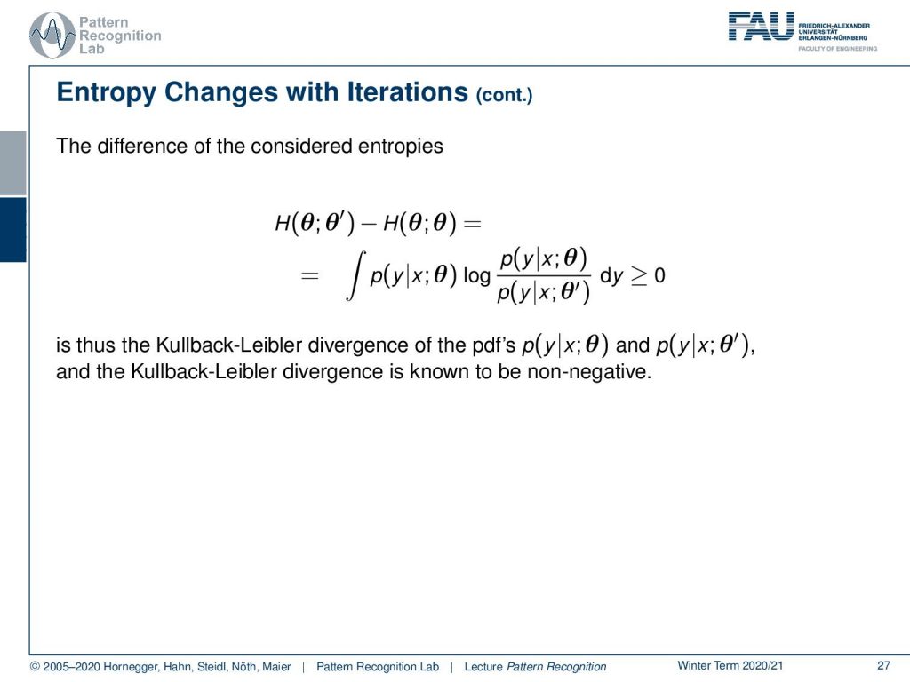
Now let’s look at this in a little more detail. What we’re computing here is the Kullback-Leibler divergence of the pdf’s of p of y given x and parameter set θ and p of y given x and parameter set θ′. So we already know that the Kullback-Leibler divergence is non-negative.

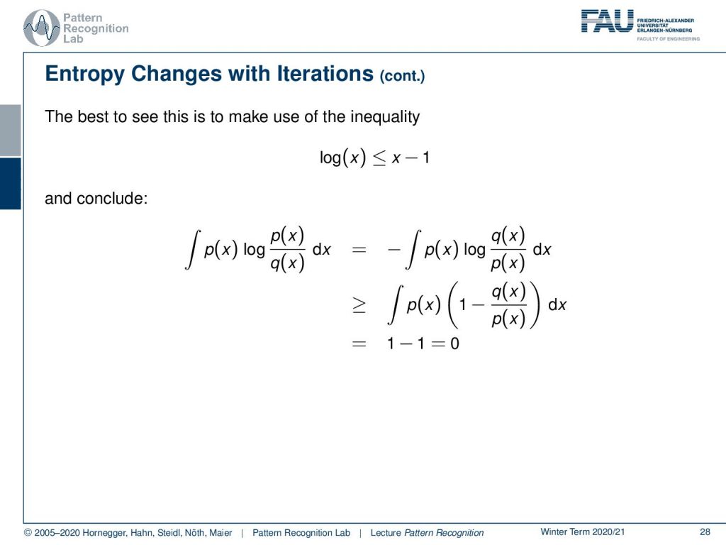
Still, we can have a little more look into these equations. We can see that quite easily if we make use of the inequality that the logarithm of x is always lower than x minus one. And now we can look at the definition of the Kullback-Leibler divergence. Again, we can use the trick that we flip the fraction to flip the sign. Now let’s use the above inequality where we know that x minus 1 is always greater or equal to the logarithm of x. Then we see that the term here will always be lower or equal to the term on the left-hand side. Now we can essentially split this integral and see that we are essentially integrating over the first term, which is essentially an integral of p(x) over the entire domain of x. We also get an integral over q(x) over the entire domain of x which is also one. So we are subtracting 1 from 1, which is equal to zero.

So we can say that the basic idea of the expectation maximization algorithm is that, instead of maximizing the log-likelihood function on the left-hand side of our key equation, we maximize the Kullback-Leibler statistics iteratively while ignoring the entropy term.

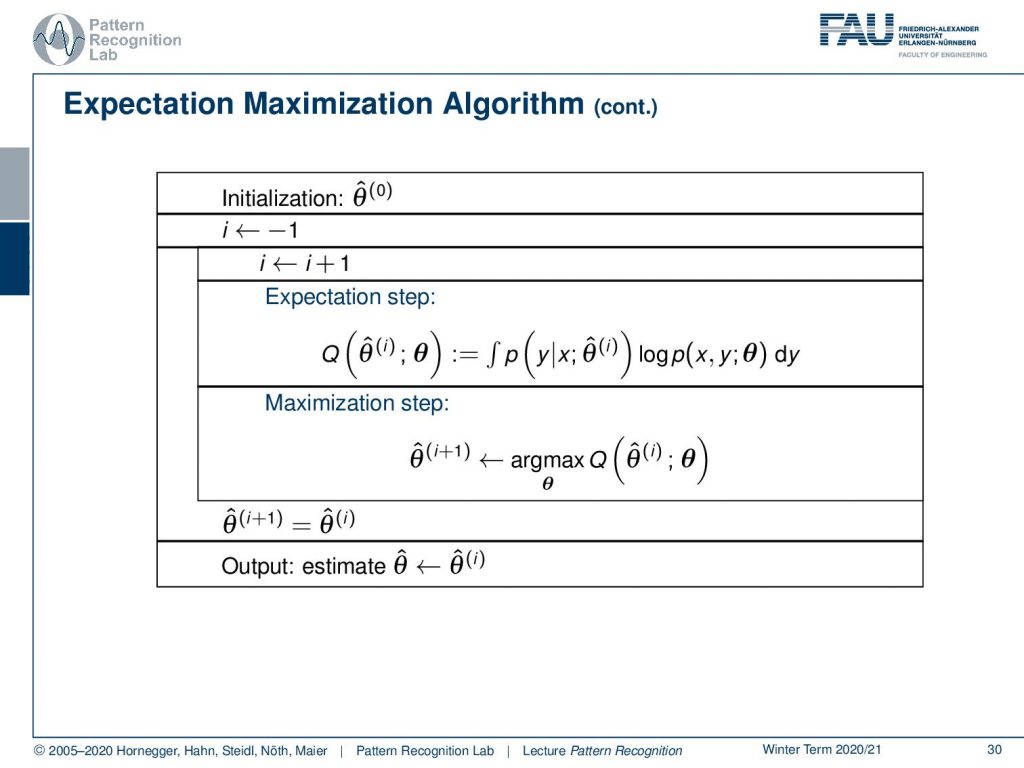
The algorithm that then emerges from this is that you start with some initialization of our parameters θ. Then we set the iteration indices and we start with the expectation step, where we essentially compute the Q function as the integral over the probability of y given x, and our old parameter set times the logarithm of p of x and y given θ. Then we compute the maximization step, where we compute essentially the update for our parameter θ⁽ⁱ⁺¹⁾ as the maximization over the Q function with respect to θ. Once we did that, we can update and iterate until we get a final estimate when the change in the parameter vector is only small.

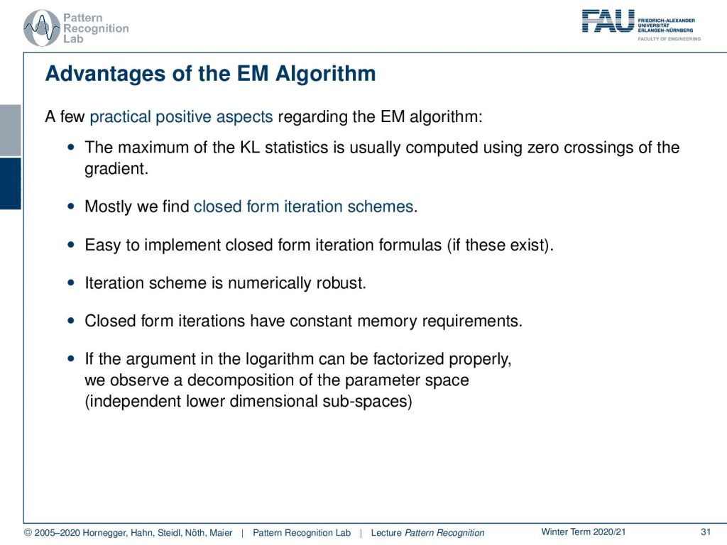
There’s a couple of advantages of the expectation maximization algorithm. It has very practical implications. The maximum of the KL statistics is usually computed using zero crossings of the gradient. Mostly, we find closed-form iteration schemes. Then, if closed-form iteration formulas exist, they are also easy to implement. And typically the iteration scheme is numerically robust. Closed-form iterations have constant memory requirements, which is also a big advantage. And if the argument in the logarithm can be factorized properly, we observe a decomposition of the parameter space. This means that we have independent lower-dimensional subspaces.

Now the EM algorithm of course also has a couple of drawbacks. And one particular one is that it has a very slow convergence. So you should not use it in runtime critical applications. Another one that is it’s a local optimization method, which means that the initialization is crucial because it essentially determines that kind of maximum that you’re converging to. So if you start in the vicinity of the global maximum, you will converge to the global one. If you start in a local lobe, then you will converge to a local maximum. This is generally a problem with the EM algorithm. 

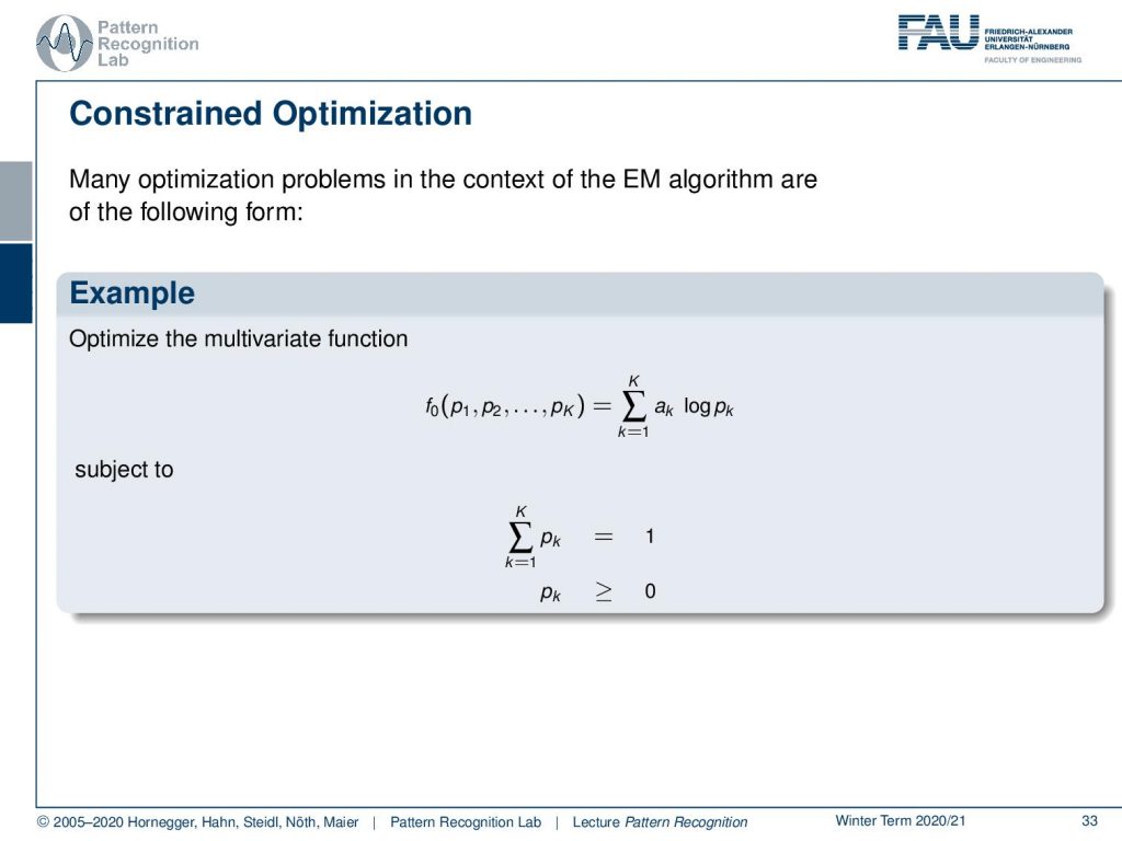
Now what we can also do is use constrained optimization in the context of the EM algorithm. This then takes the following form. So you start with a multivariate function that is given as some probabilities p₁ to p_k. Then you can essentially determine this function as a linear combination using mixture weights a_k of these logarithms of the p_k. Now generally, our p_k has to sum up to 1. Furthermore, the individual p_k has to be greater or equal to zero. 

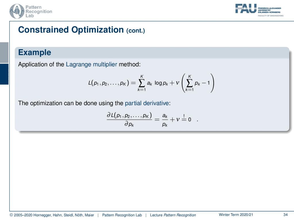
If we do that, then we can use our Lagrange multiplier method, and we can essentially put the constraints into our optimization function. This means we have the linear combination of using the a_k’s of the logarithms of the p_k’s. Then we introduce ν as a Lagrange multiplier and then we introduce that the sum over the pk needs to equal one. Now we can use the partial derivative for p_k to solve this. This then essentially leads to the a_k over p_k plus the Lagrange multiplier needs to equal to zero.

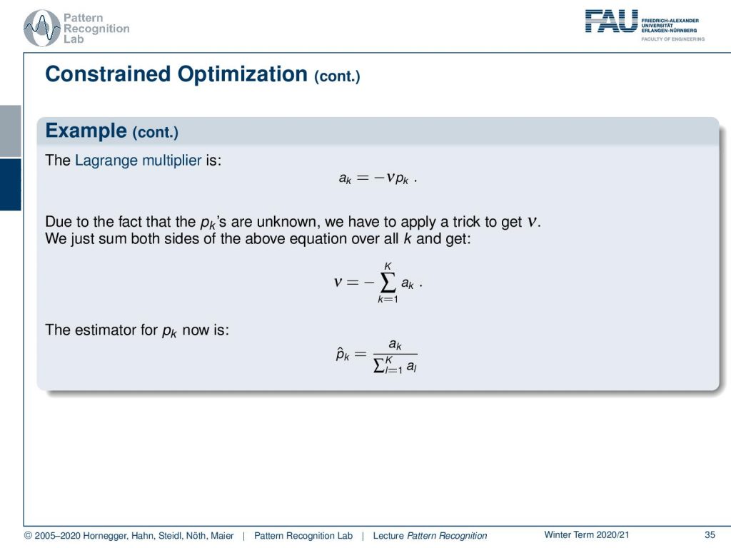
If we do that, we can rewrite it in the following form. So a_k equals to the negative Lagrange multiplier times the p_k. Now we can use a trick. We integrate over all of the k’s of this equation, and this then yields to the solution that we can solve for the Lagrange multiplier. The Lagrange multiplier is simply the negative of the sum over all the a_k. If we now put this back into our previous equation, this then allows us to find the estimator for p_k as p ̂_k  equals a_k divided by the sum of all the other a.

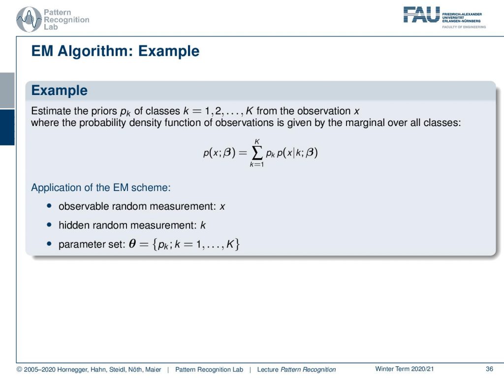
Let’s have a look at an example. The priors p_k of classes 1 to K from the observation x can be expressed as a probability density function. We write this up as the marginal over all the classes. So we see that p of x and β is given as the sum over the p_k and the probabilities of x given k. Now we can, again, here apply the EM scheme. So we have some observable random measurement x, we have a hidden random measurement k, and a parameter set θ that is consisting essentially of the p_k’s where we start from k equals 1 to K. 

Now let’s look into the idea of clustering again. For illustrating this, we consider three classes. Here we have 2D point clouds and they are labeled by colors to represent the different classes. You can see that the priors are easily estimated by their relative frequencies. Now the problem appears quite difficult if the color is missing. And this is essentially the case where we want to use our missing information principle. 

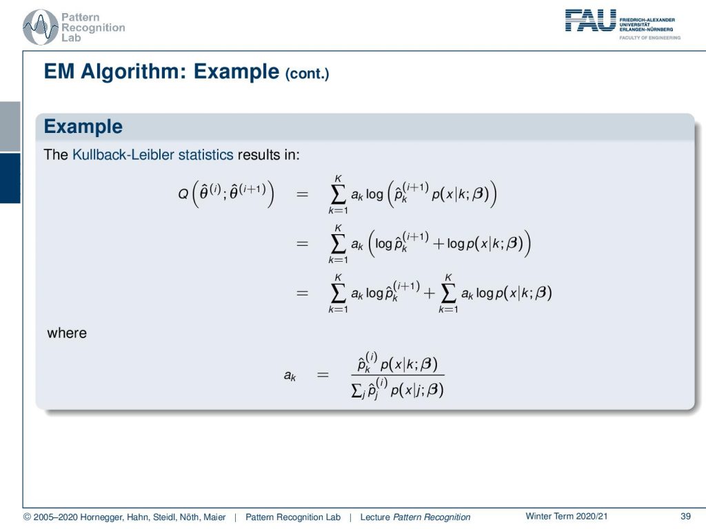
We can now compute the Kullback-Leibler statistics as Q of θ hat of i and i+1. Here this is then the sum over the a_k times the logarithm of the probability at iteration i+1 and the probability of x given k. Now we can essentially rearrange this by bringing in the logarithm and writing the multiplication as a sum. Then we can also split the two sums where we then get the sum over the aks times the logarithm of the new pk plus the sum of the aks times the logarithm of p of x given k. In our example, the a_k’s can be computed as some p ̂_k in iteration i times p of x given k over the sum of the p_j at iteration i times p of x given y.

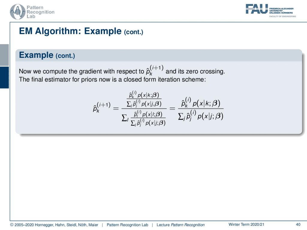
Now we can essentially reuse our previous solution scheme, where we compute the gradient for p̂_kat iteration i+1 and compute the zero crossings. This means that the final estimator for the priors can be determined in a closed-form iteration scheme. So here we get p ̂_k at iteration i+1 as this large fraction. And now you can see that this can be simplified further because the summing terms here appear twice. And this then means that you can essentially get rid of them and simplify to this equation.

Now typically, you need to initialize your priors. And what you can typically do is take application domain knowledge. So let’s say you’re working in the medical domain, then it’s the knowledge about the frequency of tissue classes. If no prior information is available, you can assume the uniform distribution.

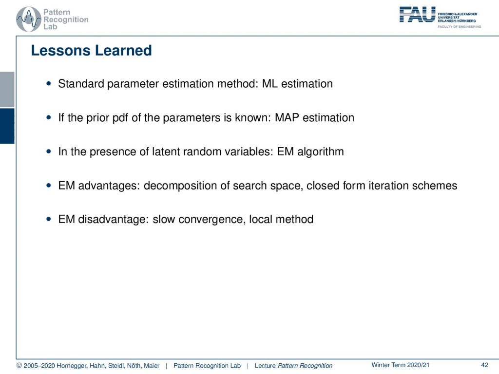
So what are the lessons learned? Well, there’s a standard parameter estimation method that is the maximum likelihood estimation. If a prior probability density function of the parameters is known you can use map estimation. Map estimation is also great, you introduce regularization, which is essentially then boiling down to the same idea. In the presence of latent random variables, you can also pick the expectation maximization algorithm. The advantages are that you can decompose the search space, and often there are closed-form iteration schemes. The disadvantage is it has a slow convergence and it’s a local method.

Next time in Pattern Recognition we want to talk about an application of the EM algorithm for image segmentation and simultaneous bias field estimation. I think you will see that this is actually a pretty cool approach, where you can then estimate this hidden information.

I also have some further readings for you. “Tutorial on maximum likelihood estimation” is very good. Then the classic introduction to the EM algorithm is the paper here by Dempster, “Maximum Likelihood Estimation from Incomplete Data via the EM Algorithm”. And of course, also “Numerical Recipes” is an important resource for us.

I do have some comprehensive questions here. What is a Gaussian Mixture Model? What is the missing information principle? And then you should also be able to write down the key equation for the EM algorithm, and you should know that the EM algorithm is generally a local method.

Thank you very much for listening to this video and I’m looking forward to seeing you in the next one! Bye-bye.

If you liked this post, you can find more essays here, more educational material on Machine Learning here, or have a look at our Deep Learning Lecture. I would also appreciate a follow on YouTube, Twitter, Facebook, or LinkedIn in case you want to be informed about more essays, videos, and research in the future. This article is released under the Creative Commons 4.0 Attribution License and can be reprinted and modified if referenced. If you are interested in generating transcripts from video lectures try AutoBlog.

References

1. In Jae Myung: Tutorial on maximum likelihood estimation, Journal of Mathematical Psychology, 47(1):90-100, 2003
2. A. P. Dempster, N. M. Laird, D. B. Rubin: Maximum Likelihood Estimation from Incomplete Data via the EM Algorithm, Journal of the Royal Statistical Society, Series B, 39(1):1-38.
3. W. H. Press, S. A. Teukolsky, W. T. Vetterling, B. P. Flannery: Numerical Recipes, 3rd Edition, Cambridge University Press, 2007.

Category: Lecture Notes in Pattern Recognition