These are the lecture notes for FAU’s YouTube Lecture “Pattern Recognition“. This is a full transcript of the lecture video & matching slides. We hope, you enjoy this as much as the videos. Of course, this transcript was created with deep learning techniques largely automatically and only minor manual modifications were performed. Try it yourself! If you spot mistakes, please let us know!
Welcome back to Pattern Recognition. Today we want to continue thinking about discriminant modeling in feature transforms. We had this idea of doing, essentially, a classwise normalization in our feature space. And if we were to do so, then certain properties in this feature space would emerge that we want to have a look at today.
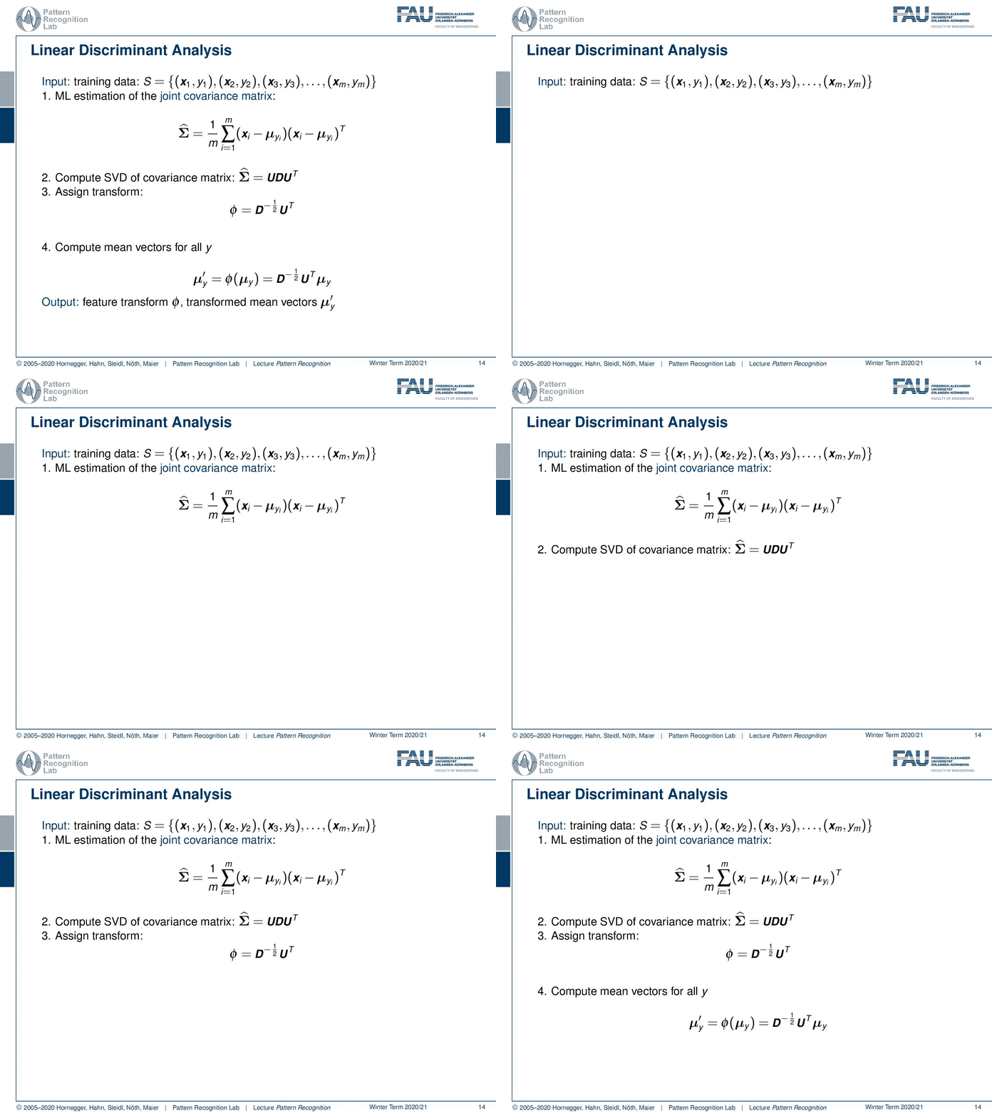
This is essentially the pathway towards linear discriminant analysis. We have some input training data that is now not just associated with feature vectors, but we also have the class labels. If we had the class labels, then we could essentially apply the transform as we already talked about. Let’s see how we could apply this to find a transform that models the different distributions of the classes differently. Well, the first thing that we need to do is to figure out the joint covariance matrix. So here we are looking into all of the observations. We compute just a single covariance matrix over the entire set. But of course, we regard the class membership by essentially normalizing with different means. So we compute the means for the different classes, and then we compute a joint covariance for all of the feature vectors, which essentially computes the variance to all of the observations. They are, of course, compared to their respective class means. This gives us a joint covariance matrix Σ̂, and now we can use our trick of Σ̂ that can be decomposed into UDU ᵀ. This then allows us the definition of a transform Φ that will enable us to map into this normalized space. And this normalized space would then be given as D to the power of minus 0.5 times U ᵀ. If we do so, then we can apply this again on our means and we get essentially the normalized means. These normalized means would be given as μ′. μ′ is essentially simply the application of the transform. So now we have the feature transform Φ and the transformed mean vectors μ′.
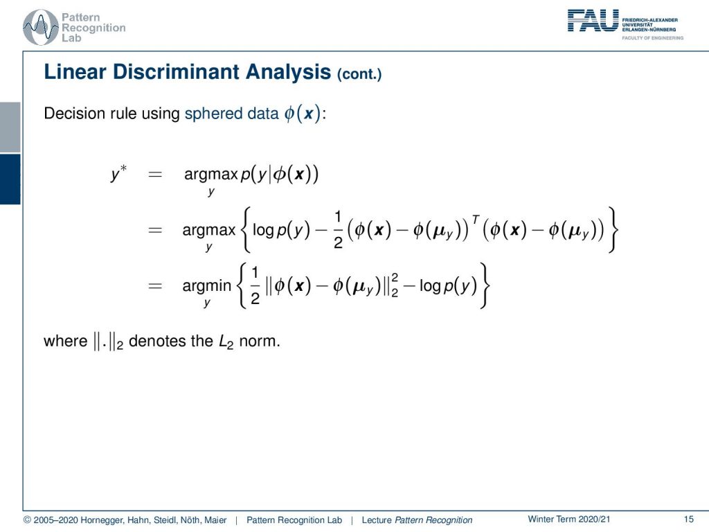
Now let’s look into the actual decision rule on this sphered data as you could say. Here then we would have our y, and here then we would have our y*, which is again maximizing the posterior probability. Now we use again the trick of decomposing the posterior into the prior and the class conditionals. Here, we already know that we’re going to use a Gaussian. So we apply the logarithm and get rid of all the terms that are not changing the decision. So everything that is essentially independent of x has been removed in the right-hand term. Then we see, we just end up with the exponent of the Gaussian distribution. Also, we see that in this case, we have an identity matrix as covariance. So this one cancels out, and we just have the feature transform in here. What we see, if we regard this then, is we can essentially remap this inner product into an L₂ norm. So we are looking here into a comparison in a normalized space that is essentially computing the euclidean distance between those normalized points. Of course, there is still some influence given the class prior, which would essentially cancel out in the decision rule if we had the same price for all of the classes.
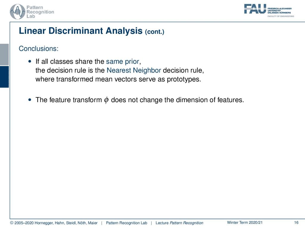
So some conclusions: if all of the classes share the same prior, this is nothing else than the nearest neighbor. And then this is nothing else than the nearest neighbor decision rule, where the transform mean vectors are used as prototypes. So we simply choose the class where we are transformed into the closest. However, also note that the feature transform Φ here does not change the dimension of the features. So here we essentially just have a rotation and scaling that is applied, and this is steered by the global covariance.
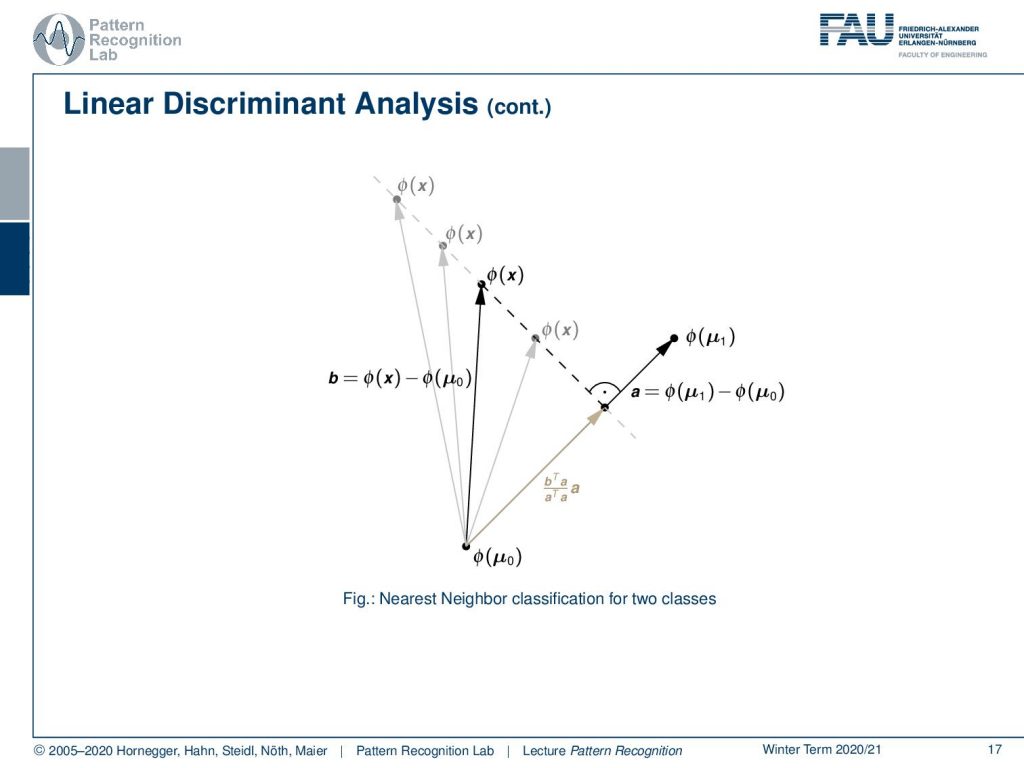
Now, let’s think about whether this makes sense or not. And I have a geometric argument here, so here we show the two means. So let’s consider the case of two classes. If I transform everything, then I’m in this transformed space. So everything here is essentially mapped by Φ. This is where I have Φ(x) and Φ(μ₁) of and Φ(μ₀). Now I can connect the two class centers, so μ₀ or Φ(μ₀) and Φ(μ₁), and this gives us the connection a. So a is the vector that is connecting the two class centers, and it’s determined simply as the subtraction of the two. This is the information that is relevant for deciding the class. Remember, our decision boundaries in this normalized space are going to be lines. Now, if I have this connection between the two, then for the classification of an arbitrary feature vector it doesn’t make any difference anymore whether it’s being moved off this decision boundary. So we can essentially take an arbitrary vector x, and then we can compute the difference between Φ(x) and Φ(μ₀). And you see that it doesn’t matter how we move it into the direction that is orthogonal to the line connecting the two means. So the class probability doesn’t change. This means that, essentially, everything that is going in this orthogonal direction is irrelevant for the classification. So maybe we could also then use this to compress our feature space.
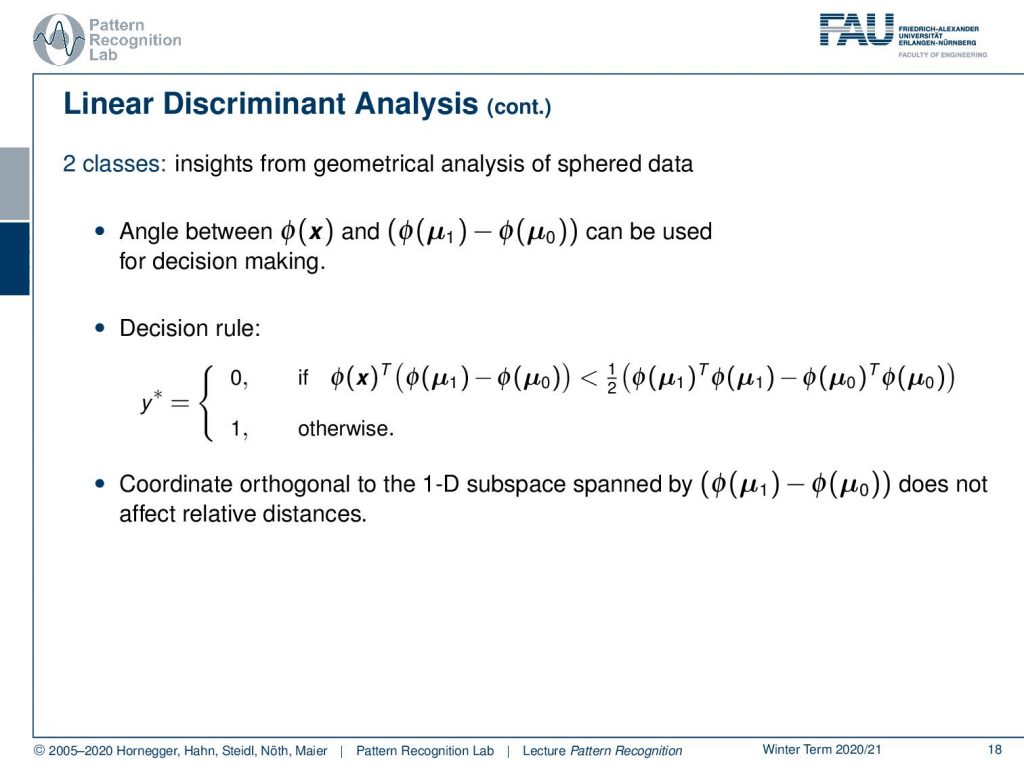
Let’s look into a little bit more detail here. You could say that, if we have two classes, then it’s really important that we essentially know the angle between Φ(x) and the connection between the two means. This can then actually be used for decision making. You see that now our decision rule is regarding the projection onto the connection of the two. So I take my transform feature vector and project it onto the line connecting the two means. And now we can simply say that if we are essentially over half of the distance, then we decide for the one class, and if we are below half of the distance, then we decide for the other class. So we can essentially neglect the coordinate orthogonal to the 1D subspace that is spanned by the connection between the two class centers in this transformed space.
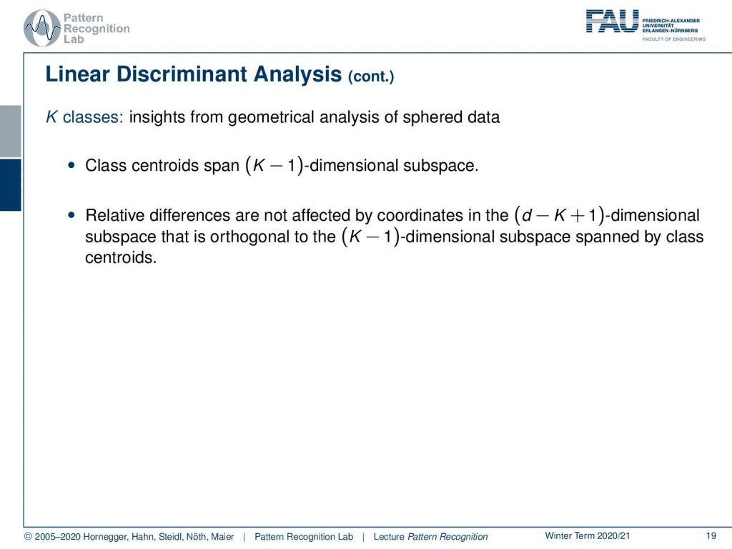
Now, we can observe from this geometrical analysis on our sphere data, that essentially our class centroids span (K-1), where K is the number of classes dimensional subspace. And everything that is not being affected by the subspace does also not contribute to the decision boundary. So, what if we have some additional dimensions? Let’s consider the case that d is higher than um k. Then in this d-k+1 dimensional subspace, the information does not contribute to the actual decision.
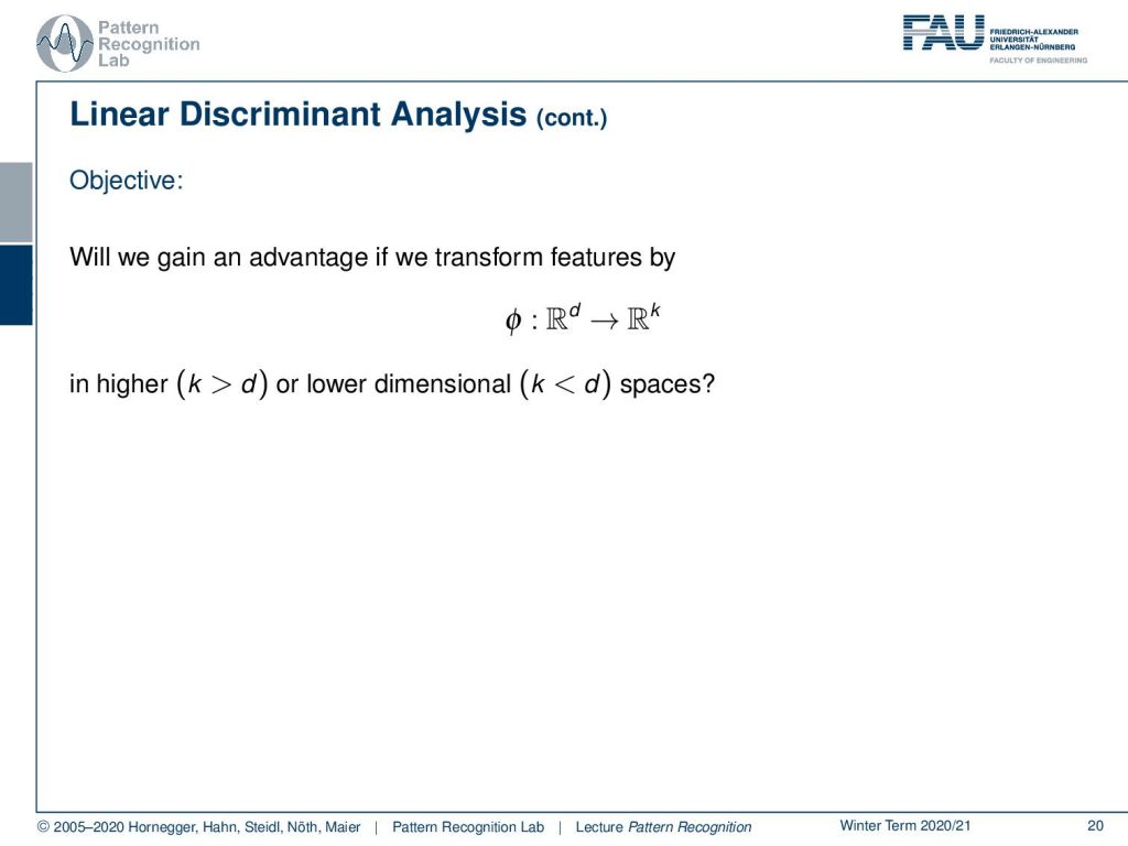
And now the idea is, of course, can we gain some advantage if we transform our features from this d-dimensional space into this k-dimensional space. The question is then also, in which configurations does this make sense. How about cases where we have more classes than dimensions? Or how about spaces where we have more dimensions than classes?
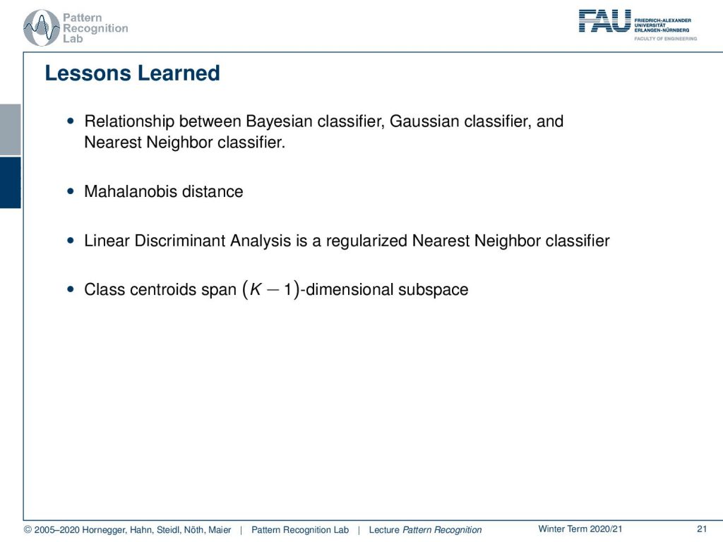
So let’s summarize this a little bit. We’ve looked into the relationship between the Bayesian classifier, the Gaussian classifier, and the Nearest Neighbor classifier. You can see that with the Bayesian classifier, we essentially have any kind of probability density function modeling. With the Gaussian classifier, we already pick a specific means of modeling the actual probability density function. And then, if we go down towards identity matrix as covariance, we essentially end up with a nearest neighbor-based classification. Also, we’ve seen the relationship between the Gaussian classifier and the Mahalanobis distance, which is essentially the case where all our classes are distributed with the same covariance matrix. And we have seen that the linear discriminant analysis is essentially a regularized Nearest Neighbor classifier. Also, a very important observation is that our class centroids span a k-1 dimensional subspace. This is, essentially, the subspace that is relevant for our classification process.

This is essentially the first considerations towards linear discriminant analysis. Now in the next couple of videos, we really want to go ahead and look into how we can actually construct this feature transform that we can then also apply to observations where we don’t have the class. So this is a very important property that, so far, for all our transformations we needed to know which mean vector to use for the normalization. And this is information that will generally not be available for an unseen test data set.
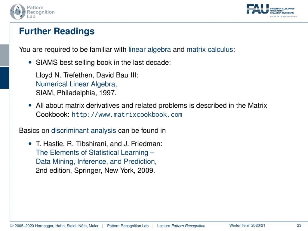
I also have some further readings. By the way, you should definitely look into linear algebra and matrix calculus if you had trouble following the things that we’ve been explaining here. I can recommend the science best-selling book in the last decade numerical linear algebra. And, of course, also have a look at the matrix cookbook. This is super useful when you’re looking into matrix derivatives and matrix manipulation. This is essentially a very good reference where you can find many important matrix identities. Also, the basics of discriminant analysis can be found in the elements of statistical learning, I really recommend also having a look into that book.
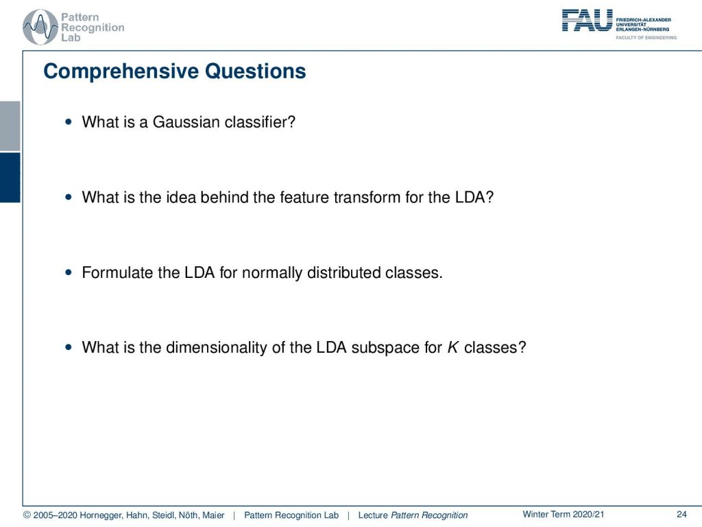
I also do have some comprehensive questions that you might find useful if you want to prepare for the exam. And this already brings us to the end of this video. I hope you also enjoyed this small presentation and I’m looking forward to seeing you in the next one. Thank you very much and bye-bye!
If you liked this post, you can find more essays here, more educational material on Machine Learning here, or have a look at our Deep Learning Lecture. I would also appreciate a follow on YouTube, Twitter, Facebook, or LinkedIn in case you want to be informed about more essays, videos, and research in the future. This article is released under the Creative Commons 4.0 Attribution License and can be reprinted and modified if referenced. If you are interested in generating transcripts from video lectures try AutoBlog.
References
Lloyd N. Trefethen, David Bau III: Numerical Linear Algebra, SIAM, Philadelphia, 1997.
Matrix Cookbook, https://www.math.uwaterloo.ca/~hwolkowi/matrixcookbook.pdf
T. Hastie, R. Tibshirani, and J. Friedman: The Elements of Statistical Learning – Data Mining, Inference, and Prediction. 2nd edition, Springer, New York, 2009.

