
These are the lecture notes for FAU’s YouTube Lecture “Pattern Recognition“. This is a full transcript of the lecture video & matching slides. We hope, you enjoy this as much as the videos. Of course, this transcript was created with deep learning techniques largely automatically and only minor manual modifications were performed. Try it yourself! If you spot mistakes, please let us know!
Welcome everybody to Pattern Recognition! Today we want to look into the actual linear discriminant analysis and how to compute it in a rank-reduced form.
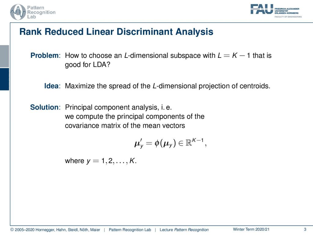
Today we go into discriminant analysis. And what we talk about today is the so-called rank reduced linear discriminant analysis. We’ve seen already that our problem was how to choose an L-dimensional subspace with L=K-1, where K is the number of classes. This is supposed to be a subspace that is good for this linear discriminant analysis. Now, the idea that we want to follow is to maximize the spread of the L-dimensional projection of the centroids. We already know a method that can do that, and this is the so-called principal component analysis. So we calculate the principal components of the covariance of the mean vectors. You remember we can transform, of course using Φ, our mean vectors. And then we can do that for all of our classes.
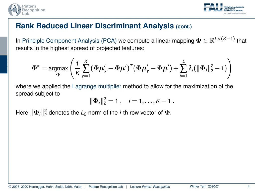
The principal component analysis, as you may know from Introduction to Pattern Recognition, is a mapping that computes a linear transform Φ. This results in the highest spread of the projected features. So this has an objective function, and here we are looking for the transform Φ* that is the maximum over this term. Now, this term may look a little complex, but you can see here this is already the version for our classes. So we take the means of our classes y, then we subtract the distance to the other means, and we essentially take the L₂ norm of these transformed matrices. Now here we type out the L₂ norm as this inner product of the two vectors. And then, of course, we compute the mean over all classes K. And at the same time, we apply a regularization. So you see here, on the right-hand side, we have some additional regularization. This is essentially a sum over the different regularization terms. And here you see that this is λᵢ times the L₂ norm of Φᵢ, where Φᵢ is essentially the eighth row vector of Φ. This essentially means that we’re looking for a matrix where the individual row vectors have a norm of one. The method that we are using to bring in these constraints, that the row vectors have a length of one, is given by the so-called Lagrange multipliers. Note that we have to introduce this kind of regularization, these constraints. Because we’re doing a maximization over the space of transforms, they could very easily maximize the left-hand side term of our maximization problem simply by maximizing all of the entries of Φ. So, if I let them go towards infinity, then I will also get a maximization of the entire term. However, this is not what we are looking for, so we need to introduce these constraints.
In case you forgot about Lagrangian multipliers, let’s have a short refresher. Generally, this is a method to include constraints in the optimization. We will use this technique quite frequently for the rest of this class. So if you have trouble with this, you may want to consult some math textbook in order to get acquainted with the concept. Let’s look into a simple example. Here, we have simply a function x + y. You already see, again as in the previous example, this is not a bounded function. So if we want to maximize x + y, we would simply go to x or y towards infinity, and that would essentially give us the maximum of this function. Generally, this is not so nice. Well, it’s actually quite easy to optimize because I can look at the function and say the maximum is at infinity. So that may be a quick solution, but it’s not very useful. So in cases like this one, you may want to work with constraints. Now the constraint that we choose as an example here is x² + y² = 1, meaning that I want to have the solutions on the circle that I’m indicating here in the plot. What I now have to do is to bring the constraint and our maximization together. This essentially needs a solution where we map our circle onto our solution space. And then, our feasible set here is indicated with the deformed circle, so our solutions must lie on that particular circle. Otherwise, we would not be fulfilling the constraint. Now, how can I bring this into the optimization? Well, one approach to go is the Lagrange multipliers. And this brings us to the Lagrangian function. Here I take the original maximization problem, and then I add the constraint with a multiplicative factor λ. This λ is then used to enforce this constraint. Now you see that our original function was dependent on x and y, and the Lagrangian function is now dependent on x, y, and λ. So λ is essentially an increase of dimensionality. And in this higher dimensional space, we can then see that all of the solutions that are solutions to our regularized problem must fulfill the constraint, that the partial derivative or the gradient for all variables needs to be zero. So you see that we compute the partial derivative of the Lagrangian with respect to x, y, and λ and set it to zero. Now you could say I could maximize the same thing in the original function by computing the partials with x and y. But we essentially introduce this additional coordinate. You will see that only critical points in this higher dimensional space, where the derivative with respect to λ equals 0, are essentially solutions on the feasible set. And if we look at the Lagrangian function, if I compute the partial derivative for λ, essentially the original objective, the x and y, will cancel out because they are not dependent on λ. All that remains is the x ² + y ² – 1. This needs to be 0, so I can solve it for x ² + y ² = 1. You see that essentially enforcing the partial derivative with respect to λ being 0 is creating a necessary condition. So, our critical places can only exist in this place if the condition is satisfied. So all critical positions in this space will have at least the necessary condition that the constraint is fulfilled. This is a very nice idea of how we can map our original problem into a higher dimensional space and solve essentially both of the optimization problems while preserving the constraint. In this particular case, as x ² + y ² = 1 is a constraint on a norm, it is very close to regularization. What you quite often see in classes that are more looking into what’s implemented and engineering solutions, is that their interpretation of the λ is some kind of engineering constant. So they just set a value for λ, of course, a value that is then chosen by the user. And you can see that any violation of the constraint in this case, so if we are not on the circle, will introduce a cost. And if you choose then λ appropriately, you essentially force solutions to be pulled towards the circle because not being on the circle will cause cost. Then, you will also more likely find solutions. Yet actually, lambda is an increase in dimensionality, and lambda is actually one of our search variables such that we can solve this optimization problem. A very short primer into Lagrangian optimization.
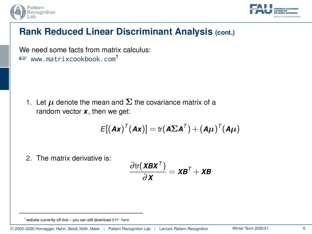
Now, let’s go back to our original problem. And one thing that I want to use in the following is two shortcuts from the matrix cookbook. Again, here the link to the matrix cookbook www.matrixcookbook.com. It should be rather easy to memorize for you guys. And here we will use the following two identities. Well, the first one is, if we have some kind of expected value that is following a mean vector μ and a covariance Σ, then we can replace this expected value and a transformation of the individual features x by a transform A. This can be rewritten into the trace of A Σ Aᵀ + (A μ)ᵀ (A μ). Also, note in this identity, if I had a normalization to μ equals to 0, so I’m forcing essentially everything to be centered, then the right-hand term would cancel out. So we would only have the trace of the matrix A times the covariance matrix times Aᵀ. Now this trace is kind of interesting. This brings us to the second shortcut, the matrix derivative of a trace with respect to A. Or in the next time this is going to be X. So if you’re actually interested in computing this partial derivative with respect to X, you see this is still a similar setup as the trace in the line above. Then this can be rewritten into X Bᵀ + X B. Now, very interesting about this is as well that if B were a covariance matrix, then the transpose would essentially not change the matrix because it is symmetric. And this way, you could even write this down as 2XB.
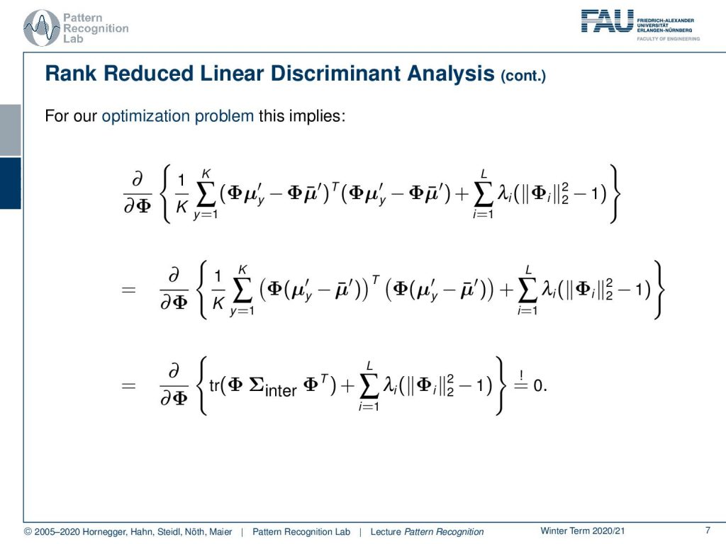
Let’s look into our rank reduced linear discriminant analysis. Here we see that we can rearrange this a little bit. So you see that our feature transform is applied to our class means and also to all the other means. This means we can actually pull this guy out. So we end up with the difference of the class means to all the other means or essentially the complete mean transform. This means that our distribution is mean free, so we have a 0 mean vector in the transformed space. This then allows us to use the previous trick with the trace. Here you see then that we simply have the inter-class covariance matrix. And then we have the trace of Φ times the inter-class covariance matrix, essentially the covariance matrix of the mean vectors, and this is multiplied again with Φᵀ. So you see the other two terms that were introduced in the matrix cookbook cancel out because our distribution is mean free in this case, which then eliminates this from our equation.
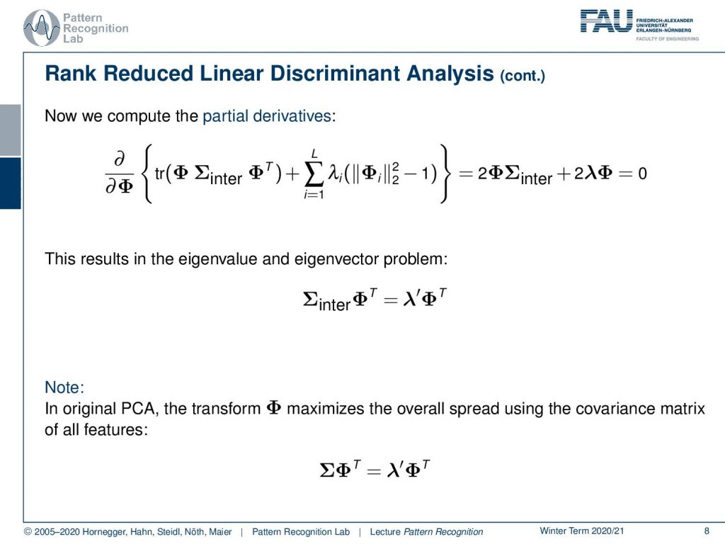
Now you see we have this trace, and we know from our matrix cookbook that we can simplify this trace by writing this up as Φ times covariance inter plus Φ times covariance inter transpose. And this, of course, we can rewrite as 2 times Φ Σinter, and on the right-hand side, we have a derivative of an L₂ norm. This L₂ norm derivative we can simply write down as two times the number of Lagrangian multipliers in a vector. And then we get our original feature transform Φ. So you see that we can simplify this quite a bit and this necessarily has to be zero. You can see that if we divide by two now, this essentially gives us the eigenvalue and eigenvector problem Σinter Φᵀ = λ′Φᵀ. Note that we essentially got rid of the minus by introducing this λ′. Have a look here, this is from the original PCA. There, the transform matrix is created by maximizing the spread over all the features using the covariance matrix of all the features. Here you essentially end up with the problem that you have Σ and then Φᵀ equals to λ′ and Φᵀ again. So again, we have this eigenvector and eigenvalue problem, and this then can be computed, of course, by simply computing the eigenvalues and eigenvectors of our respective covariance matrices. So for the rank-reduced linear discriminant analysis, you need to apply it to the inter-class covariance matrix. And in the normal PCA, you would apply it to the regular covariance matrix.
Let’s look at the steps that we need to compute our rank reduced linear discriminant analysis. So we go ahead and compute now the covariance matrix of the transformed mean vectors. In the first step from the previous video, you remember that we first apply the normalization with respect to the general covariance matrix and transform it into this normalized space. And then we compute in this normalized space the covariance over our class means. And then the mean of means is of course the mean of all the mean vectors. Now you compute the L eigenvectors of the covariance matrix belonging to the largest eigenvalues. This can obviously be done with standard eigenvalue analysis. And then you essentially choose the eigenvectors that then become the rows of the mapping Φ from the K – 1 to the L dimension of feature space. This then gives us the output matrix Φ.

That’s essentially all for today. You looked at the rank reduced form of the linear discriminant analysis. What we want to do in the next video is to look at the original formulation that is then often also called the Fisher transform. So this is essentially a variant of the LDA. I think you should know the difference between the rank reduced version that we just presented and the original transform. I hope you liked this small video and I’m looking forward to seeing you in the next one! Bye-bye.
If you liked this post, you can find more essays here, more educational material on Machine Learning here, or have a look at our Deep Learning Lecture. I would also appreciate a follow on YouTube, Twitter, Facebook, or LinkedIn in case you want to be informed about more essays, videos, and research in the future. This article is released under the Creative Commons 4.0 Attribution License and can be reprinted and modified if referenced. If you are interested in generating transcripts from video lectures try AutoBlog.
References
Lloyd N. Trefethen, David Bau III: Numerical Linear Algebra, SIAM, Philadelphia, 1997.
T. Hastie, R. Tibshirani, and J. Friedman: The Elements of Statistical Learning – Data Mining, Inference, and Prediction. 2nd edition, Springer, New York, 2009.
B. Eskofier, F. Hönig, P. Kühner: Classification of Perceived Running Fatigue in Digital Sports, Proceedings of the 19th International Conference on Pattern Recognition (ICPR 2008), Tampa, Florida, U. S. A., 2008
M. Spiegel, D. Hahn, V. Daum, J. Wasza, J. Hornegger: Segmentation of kidneys using a new active shape model generation technique based on non-rigid image registration, Computerized Medical Imaging and Graphics 2009 33(1):29-39