X-ray Photon-Matter Interaction

These are the lecture notes for FAU’s YouTube Lecture “Medical Engineering“. This is a full transcript of the lecture video & matching slides. We hope, you enjoy this as much as the videos. Of course, this transcript was created with deep learning techniques largely automatically and only minor manual modifications were performed. Try it yourself! If you spot mistakes, please let us know!

Welcome back to Medical Engineering. So today we want to talk a little bit more about x-rays and in particular what happens when the x-rays hit the body and how they interact with the tissues inside of the body. So this will be the interaction of photons on matter in a summary of all the things that can happen. 

So let’s go back to our slides here and this is part 2 of x-rays and now we will discuss the interaction of x-rays of matter.

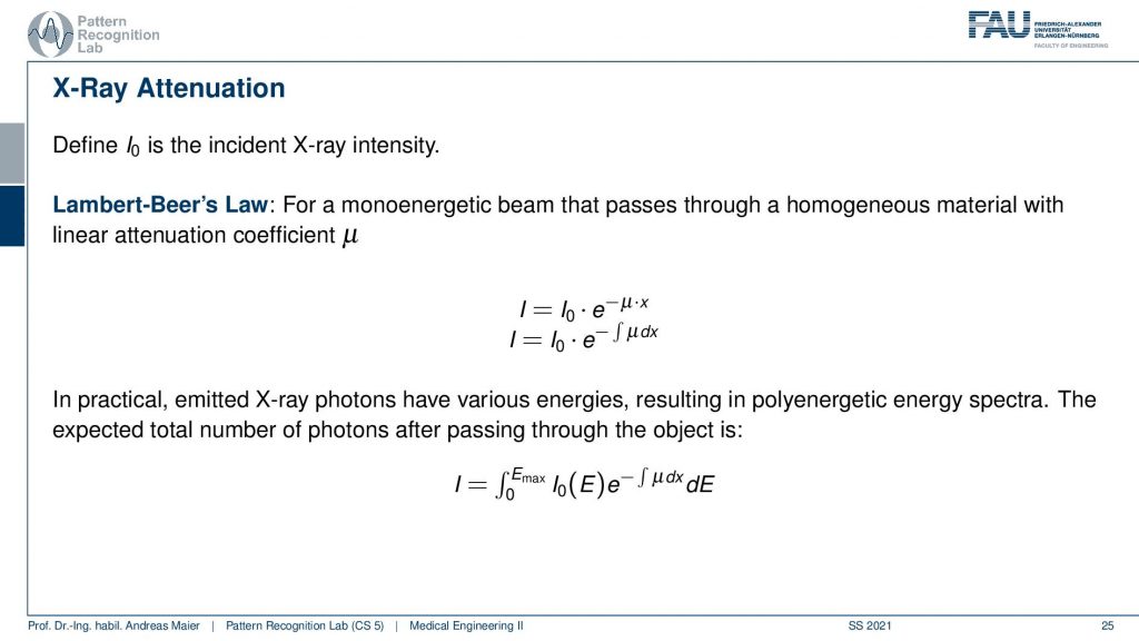
Now what happens if we have generally some x-rays interacting with matter is we get attenuation. We somehow have to model the attenuation. In order to model the attenuation, we have the so-called Lambert-Beer’s law. Lambert-Beer’s law is essentially describing the effects of what happens inside the body when the x-rays interact. So what we can see is that there is I, I_0, and this strange term here. Now, I is essentially what we observe at the detector. So this is our detector. Then we have I₀ this guy here which is the x-ray tube. It’s this guy here and this emits x-rays and the x-rays that are emitted here. This is the intensity I₀. Now what happens is that you have a patient in here and this is our patient. Then the x-rays somehow interact with the patient and this is described exactly by this term here. So what happens inside the patient is this guy and then we detect here on the detector our I. So we can write this up as this formula. You see that we have this exponential function here. The exponential function to the power of -μ times x tells us what is happening and you see here that x is nothing else than the length of the intersection of the ray of the body. So this is x, this guy here. Now μ is a characteristic constant for the material. So let’s say this is the material. Let’s say it’s a constant material. So the patient consists completely of water. Then you can write material constant μ. So this is the x-ray absorption times the path length and this will give you a coefficient and if you take this coefficient e to the minus this coefficient it will give you essentially the probability of the x-rays being absorbed. This will give you a reduction of the original x-ray intensity that is then observed in the detector. Now typically we don’t have only one tissue. So typically we have many different tissues here, right? So there’s a liver and there are different organs and they all have different x-ray absorption. This is actually why we do it. If they all had the same x-ray absorption then we could only measure the path line. So instead what is happening here is that we have an integral. So you could say that along the body if this is x then the μ at the position x is changing. Let’s say this is the liver and this is the kidney and this is some other material and here’s a bone. Then we have a very high μ. Then what’s happening is that you’re no longer just multiplying the path length with the constant but instead, you’re measuring the integral. So you’re essentially measuring the area under this curve here and this determines this integral here. Then you take it to the minus and e to the power of minus this integral and this gives you essentially the absorption probability. So this is how you can understand Lambert-Beer’s law. So it is a function that tells you how much of the energy will get absorbed within the body and this is dependent on the tissues and it’s dependent on the location. So that specific tissue at that location. Now you already see that this is interesting because this profile that I’ve been drawing here is nothing else than the intensity profile or the density profile along this line. Now you can also understand that we are kind of measuring the integral, superposition of everything. It’s a bit stupid because this integral is up here right? So we can’t measure this directly. So now you could argue how can I actually solve for this integral? You can see that this can be done rather easily if we look at this equation here then we see if we now divide by I₀. So we take I over I₀ and then we take the logarithm natural logarithm and then we multiply with minus one. You see that is the left-hand side of the equation and on the right-hand side of the equation, we have only the integral of μover the path of our x-ray. So this is why I said earlier look we are measuring the integrals because I know the tube settings, I know how many x-rays are generated and I detected the other side how many of these x-rays actually arrived at the detector. So everything on this side here is known and of course, the logarithm and the minus is something that I know and all of the unknowns there on this side here. This means that I’m measuring line integrals along with the x-rays. So that’s a cool property and we’ll see that this is essentially the key property that will allow us to generate the so-called computer tomography. How we can virtually cut our patient into slices similar to MR that we’ve already seen. We also see that we need a little more mathematics in order to understand computer tomography which is essentially the reason why we’re discussing MR imaging before x-rays. Although x-rays have been discovered much earlier. But we will see that the mathematics of MR essentially date back to the Fourier transform that was discovered 250 years ago. The actual inversion for computing computed tomography was only discovered in 1997. But we look into the details when we talk about computed tomography. Now also the reason why computed tomography is not that easy is we have many different energies. So actually our intensity is not just dependent on Lambert-Beer’s law here. But it’s embedded in this kind of integral here and this is an integral over the energies. This messes up most of the reconstruction formulas and therefore we then have to solve them with different solution strategies in order to be able to compensate the energy-dependent. Well, we’ll look into that more in later videos. So let’s not get confused by the multi-energetic nature of the x-rays here we just want to show you this and we will look into more details of the multi-energetic part also in this video.

One thing that we should talk about is how this μ is actually composed.

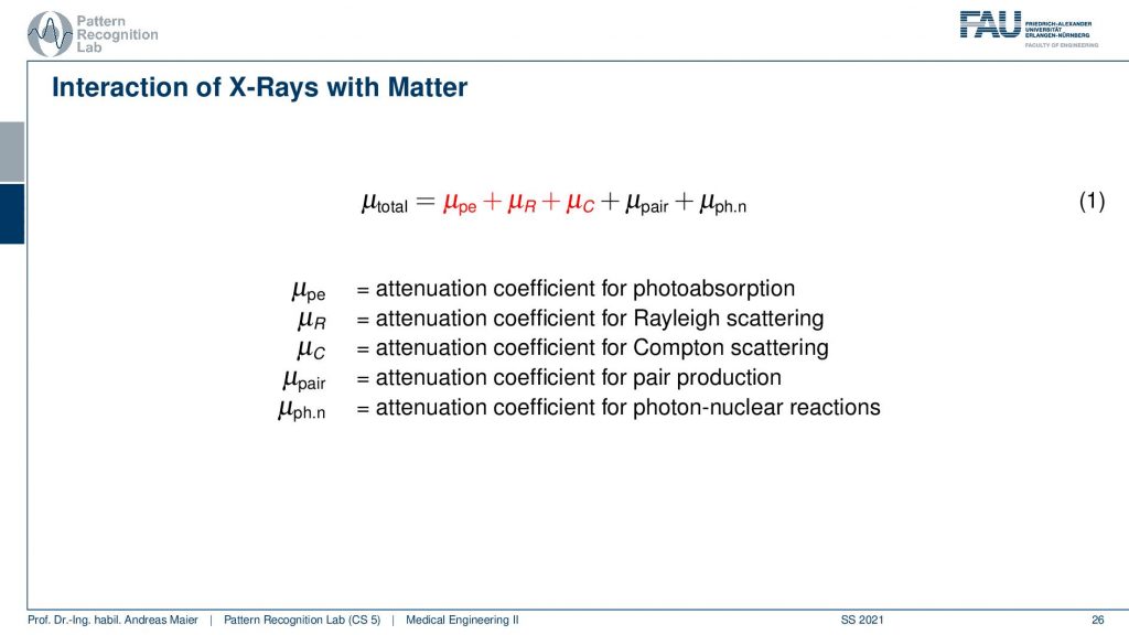
So I talked about μ and said it’s a material-dependent kind of characteristic. It tells us that it’s the liver or something like that but there’s actually more to that. It’s not just μ. It is composed of a series of different effects. so there is μ_pe which is the photoabsorption there is μ_r which is the Rayleigh scattering and there is μ_c which is the Compton scattering. So those three effects are relevant for most of the x-ray imaging. There are additional coefficients that might play a role but this is then the absorption caused by pair production and also photon nuclear reactions and this doesn’t happen at the energies when we’re actually talking about x-ray imaging. So this happens beyond 200 kilovolts and above and therefore we don’t have to consider these effects here. So let’s look into the red ones here because these are the ones that are relevant for x-ray imaging. 

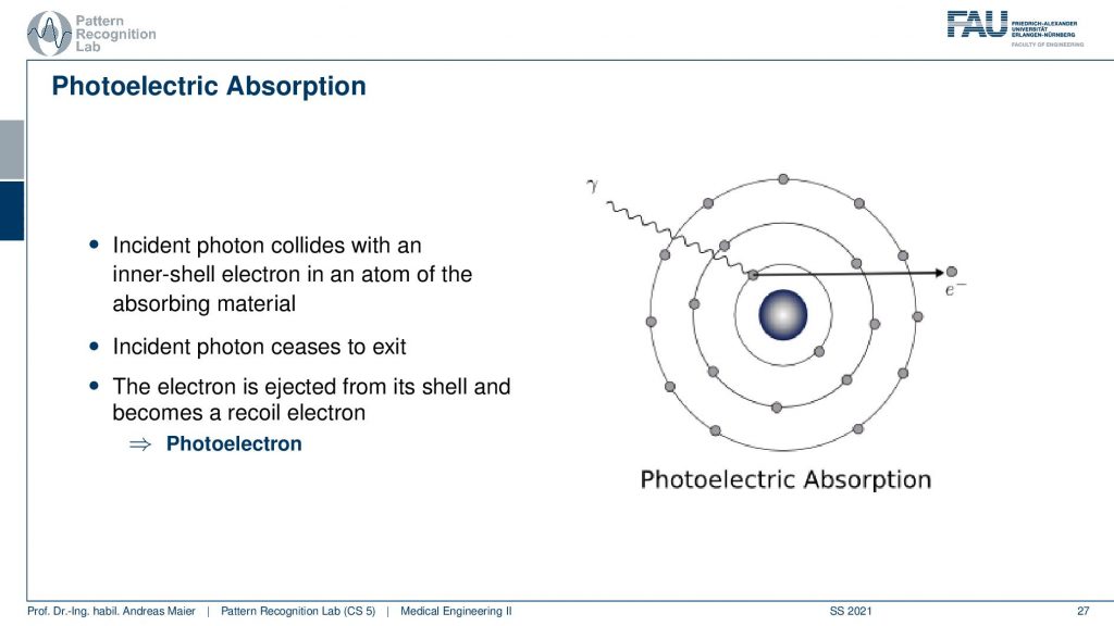
Now there is the photoelectric absorption. The photoelectric absorption is now happening when the x-ray is kind of entering the shell of the material under investigation and it can hit essentially an inner shell electron and this is ionized. So x-rays are ionizing radiation. Here we have a change of the atoms under investigation and the ionization is also the reason why we actually have a breakdown of DNA and stuff like that. So this is why x-rays are a pretty kind of risky kind of method to look inside of the body. But still, if you use only very few x-rays not too many of these ionizations happen and we assume that the risk of cancer is linear with the amount of energy deposited in the body. So here you collide with an inertial electron and the electron is being ejected and we have ionized this material here. This is then a photoelectron that is being emerged. So this is one effect that can appear and then of course the energy of our photon here is completely absorbed. Now, what can also happen?

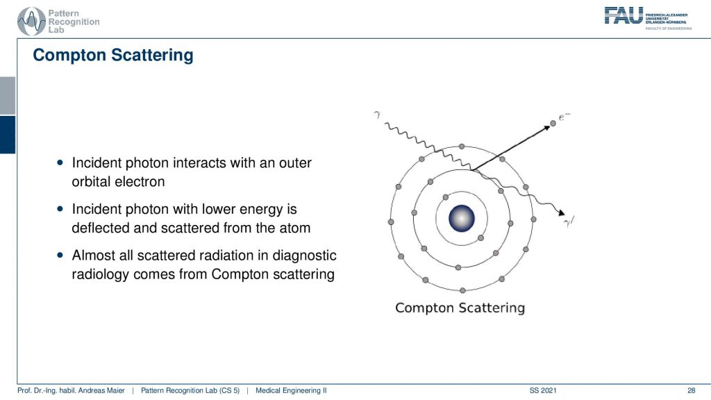
There is the content scattering. It is a kind of interaction that happens if you are interacting with the shells. So you have an incident photon that interacts with an outer orbital electron. Then the incident photon with lower energy is deflected and scattered from the atom. We observe that almost all scattered radiation in diagnostic imaging comes from content scattering. So we have this photon coming in. Then it’s emitting this electron here and it continues in a different direction with a longer wavelength which means that it has reduced energy. So this is the content scatter and it’s the main cause of absorption inside the human body.

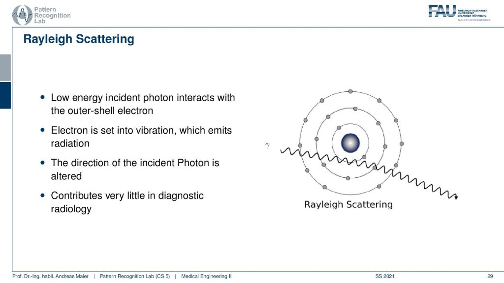
There’s a third effect that’s Rayleigh scattering. Rayleigh scattering is that we have a low energy incident photon interacting with an outer shell electron and the electron is set into vibration and because we vibrate the electron it emits radiation. So then we kind of see that it changes the direction of the incident photon and this is a kind of deflection process. So we have a wavelength coming in and then we see that the direction is altered and we have a change of direction. This contributes only very little to diagnostic imaging. But this way we are able to describe certain deflection effects that appear and this also reduces the energy of the photon along its path.

Let’s have a look at the energy dependence.

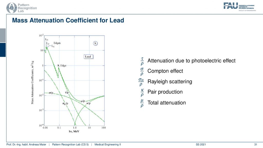
We see that here in this very nice plot we see that we have the energy of the photons and we have the attenuation coefficients in this direction. So we see that depending on the energy we get a different attenuation coefficient. So if I use higher energy you can already observe that generally, the absorption coefficients here go down. So you see here that our absorption coefficient goes down which means the higher the absorption it is more likely that this photon is being absorbed. What we can also see here is that we have different effects that are being described in this kind of figure. You see for example that the effect of pair production only emerges here. So you have to be essentially beyond 1 MeV for the pair production. Then you also see the total attenuation. The total attenuation is this guy here and what we also see you see these nice edges. This is called the K-edge and the K-edges are essentially determined by the material. What can we also see here? This is lead right and here you generally see really high absorption coefficients because lead is very dense and essentially two millimeters of lead shield any kind of diagnostic x-ray source. So two millimeters of lead is sufficient to be safe and this is, of course, the reason why we use lead shielding in interventional applications of x-rays such as no x-rays actually can penetrate your body. Two millimeters of lead and that’s enough. Then we can see that dependent on the effect. So this is the Rayleigh scattering and you see that the Rayleigh scattering is actually following this curve here. So in diagnostic, it’s not such a big thing and then we see the Compton effect which is happening here. So this is Compton and this is essentially the dominant kind of absorption. Then of course we have on top the photoelectric effect and let’s use this color for the photoelectric effect and you see here the photoelectric effect is the one that introduces the K-edges. Because there we are ionizing certain shells in the hull of the atom and here we then see again that we have characteristic steps emerging exactly at the energies where the characteristic steps in the shadow actually occur. Okay so let’s compare that with for example water.

You can already see here is that we have a much lower. So it’s still the same energy range but we have an order of magnitude lower absorption in this plot. So it’s very careful that you actually look at the absolute numbers here and here if you want to compare the previous and this plot to observe that this is very different. What’s also different in this plot is that we see that we have the total absorption here and again we see for example that there are no K-edges here. So with water, we don’t observe K-edges and it’s of course because we have very simple hulls. So this is hydrogen-oxygen and we don’t have too many shells here. So we don’t observe the K-edges in the photoelectric effect and then we also see that the Rayleigh absorption also doesn’t play such a big role and this is the Compton scattering. So you see that in different materials we, first of all, have a different distribution of those effects. So the Compton photoelectric and also the Rayleigh scattering is different in every material and we can characterize this in plots and we also see all of this is energy-dependent. So depending on the energy, the effects mix differently. So this is interesting because now if I observe characteristic energies or distinct energies. So let’s say I observe the energy here and the energy here and I do that for another material as well. Then I can characterize the materials from the difference in the absorption characteristics dependent on the energy and then this gives rise to material separation. This is essentially a similar approach as we’ve seen already in MR that we had this water-fat separation. Similar things can be constructed here with x-rays. We can then differentiate let’s say water and iodine or any two kinds of materials that are different in their absorption behavior for the particular energies that we investigate.

So this brings us already to the end of this video and in this video you understood how x-rays are actually interacting with matter. We’ve seen that there are essentially three major effects that happen and these are three types of scattering. We’ve seen that is the photoelectric effect, the Compton effect, and the Rayleigh scattering. Another thing that we observed is that when we describe the entire attenuation of the x-ray we can see that this is essentially the initial intensity multiplied with this term that is this e to the power minus the integral through the line through the body. We have also seen that if we know the detected intensity and the emitted intensity then we can solve for this line integral which essentially allows us to understand the x-ray image as a kind of sum as a kind of superposition of all of the contents of the body into a single image. This will be very useful when we talk about computed tomography. So I hope you enjoyed this video and understood a bit about the physical effects that actually govern the underlying contrast mechanism of x-rays. Now in the last video regarding x-rays we want to look into the actual absorption and what’s actually happening when we detect the x-rays on the detector. So I hope you enjoyed this video and I’m very much looking forward to seeing you in the next one. Bye-Bye!!

If you liked this post, you can find more essays here, more educational material on Machine Learning here, or have a look at our Deep Learning Lecture. I would also appreciate a follow on YouTube, Twitter, Facebook, or LinkedIn in case you want to be informed about more essays, videos, and research in the future. This article is released under the Creative Commons 4.0 Attribution License and can be reprinted and modified if referenced. If you are interested in generating transcripts from video lectures try AutoBlog

References   

Maier, A., Steidl, S., Christlein, V., Hornegger, J. Medical Imaging Systems – An Introductory Guide, Springer, Cham, 2018, ISBN 978-3-319-96520-8, Open Access at Springer Link

Video References

1. X-ray projection of the Hand https://youtu.be/OY3RufOylek
2. AP & Unilat AP Oblique Projection https://youtu.be/wlyeSA4zzU8
3. X-ray Material Decomposition https://youtu.be/XGXpIX8gPWc

Category: Lecture Notes in Medical Engineering