X-Ray Detection

These are the lecture notes for FAU’s YouTube Lecture “Medical Engineering“. This is a full transcript of the lecture video & matching slides. We hope, you enjoy this as much as the videos. Of course, this transcript was created with deep learning techniques largely automatically and only minor manual modifications were performed. Try it yourself! If you spot mistakes, please let us know!

Welcome back to medical engineering. Today we’ll look at the third part of X-rays and we want to discuss the actual detection of the X-rays on certain kinds of X-ray sensor technology. So now let’s have a look at our slides.

So now we want to discuss the actual imaging and it is the last part in the chain. 

So we had the generation. We had the interaction with matter and then we want to convert now the X-rays into something that we can then display as an image. So we will discuss the following image intensifiers and flat-panel detectors. So these are two key technologies that are being used to detect. Nowadays most systems use flat-panel detectors. But I think if you see an image intensifier you should know how it works. This is why we still have it here in the set of slides and then we want to discuss shortly the sources of noise in X-ray imaging.

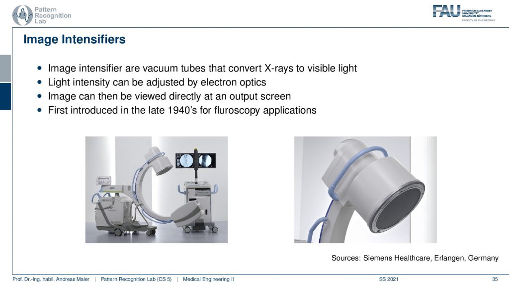
These are the X-ray image intensifiers and they are essentially vacuum tubes that convert X-rays into visible light. The nice thing is that we can adjust the magnification in these systems on top. So there is electron optics that we look into in a couple of slides and they allow us to essentially zoom in and zoom out continuously. This is also why this technology has been very popular for a long time because if you have a flat panel then you can only work with different binning and the difference is essentially like in your camera where you have the optical zoom where you can continuously zoom in and zoom out and then you have the digital zoom which is essentially either causing interpolation or you have to jump in discrete steps because you bin you summarize a certain number of pixels. So first these image intensifiers have been introduced in the late 1940s for fluoroscopy applications. So fluoroscopy is generating entire movies of X-rays and therefore you have to have a very high sensitivity and the image intensifiers were able to make the usable signal for display much more efficient. Therefore you could reduce the X-ray dose which then allowed to produce entire X-ray movies and the X-ray movies are still called fluoroscopy. 

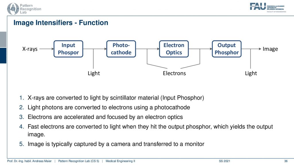
Now, what’s happening in such an intensifier. You generally have a couple of steps of conversion. First, you have an input Phosphor. The Phosphor generates visible light from the X-ray. Then the photocathode is then generating from the light electrons. The electrons are then being accelerated through electron optics. This is then hitting some output Phosphor and the Phosphorus glows again when the electrons hit and this causes light and this light is then measured. So this is the schematic.

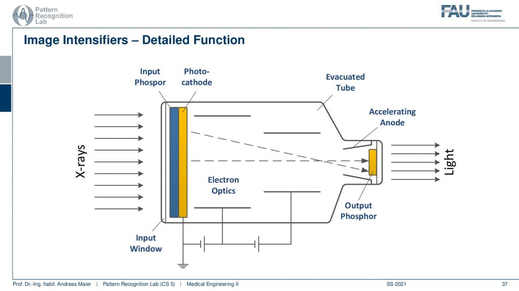
Let’s look into a more generating approach here and here’s you see that actually the input Phosphor and the Photocathode. There are two layers directly behind the screen. So you convert from X-ray to visible and from visible directly into electrons and then you use a voltage here and this voltage is used to accelerate the electron in order to increase the intensity and to harness more signal. Then because you have essentially electrons passing here towards your detector like the next Phosphor then you could use electron optics to adjust the beam. So you can essentially focus it or spread it more and this is done with these electron optics. All of this is embedded in an evacuated tube and finally, you hit the output Phosphor and then you get the light. The light can then be either displayed or it can also be digitized and then you have a digital image. So these are the classical image intensifiers. 

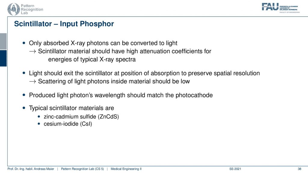
So if you look this into the individual parts you see that there is the Scintillator which is the input Phosphor and it has also a certain characteristic. So the Scintillator material then is essentially describing how well the X-rays are transformed into visible light and this again has a characteristic. So far we only were interested in the contrast that is caused inside the patient. But actually, that’s not entirely true. We also have an additional loss of signal in this conversion process in the detector. Therefore you want to choose the scintillator material such that they are optimally designed for your specific application and there are two types of Scintillator materials. There’s the zinc cadmium sulfide the ZnCdS and there’s the cesium iodine the CsI detectors and the main difference here is the absorption. 

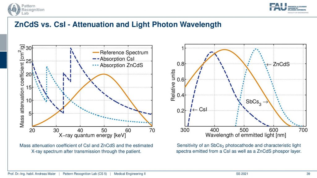
So here you see a reference spectrum. So this is the distribution of the X-rays that we expect to arrive at the detector. Then you see that if I choose the zinc cadmium sulfide then I actually have this conversion curve. If I choose the cesium iodine then you see I have this conversion curve. So the overlap in this region is much better for the cesium iodine and they get a much better signal and this is then a key reason how to select actually the Phosphor material and you wanted to prick it in a way that suits the specific application. If I had lower X-ray spectra so if my reference spectrum would look like this then I would probably prefer the zinc cadmium sulfide. So you see that this is crucial when designing your system that depends on the energies that you’re expecting you want to use different materials for the Phosphorus. Then there’s another effect that’s happening. This is the generation of the wavelengths. So you see this is essentially visible light. Now you see that the light that is generated here is different for the Cesium Iodine or for the zinc cadmium sulfide which is here. So that’s also a property that you have to be aware of when selecting then essentially the next step in the conversion process because you want to convert this to electrons right. So you also have to be aware of these properties of your Scintillator. 

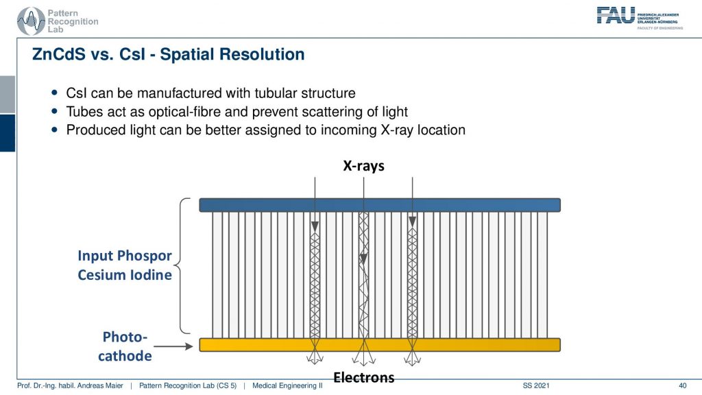
Now if we want to assemble this then what’s also very important is how the X-rays hit your detector. So let’s say we have some Cesium Iodine Phosphor. Then the cool thing is it’s made with crystals. So it has a crystalline structure and you can grow very long crystals here. Now what happens is if your X-ray comes in here and it’s being converted into visible light it will follow this signal structure and then here the photo cathode will convert it into electrons. This is pretty cool because my X-ray could also hit very early or it could hit very late in the material and because we have this crystalline structure and now we have visible light that gets reflected right. So it stays within those tubes here. If you had none of these tubes what then would happen is of course that it would just spread in a certain point spread function and you see then if we have an interaction here we would have much more blurring than if we have interaction here. So that’s really cool that we have these crystalline structures when converting into the light and into the subsequent electrons. So this is pretty cool!

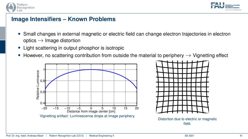
One problem with image intensifiers is what quite frequently happens is that you have a certain bending of the input Phosphor and this then causes a change in the geometry. What can happen here is that if your input Phosphor is bent or, if you have additional electron optics, you could have an electric or a magnetic field around. What then happens is if you had a perfect grid that should look like this. Well, it’s not a perfect grid that I’m drawing here but you remember so this should be straight lines. You can think about this and now my straight lines get projected onto curved lines. This can happen if your input Phosphor is not flat or if you have additional electrical magnetic fields. So this is pretty annoying and if you want to use this in things like CT then you have to calibrate from the geometric distortions that are introduced by your image intensifier. This being dependent on magnetic fields is also very annoying because if you build a system and you calibrate it in the factory and there are no magnetic fields around then you get wonderful images and you ship it to a customer and then suddenly you got no image at all at the customer side. This happened and then people haven’t said no it’s a defect detector. You can’t use that you bring it back to the factory and that just works fine. You have to be aware that you don’t have any disturbances in terms of a magnetic field. So if it’s there’s an MR scanner next door maybe it’s not such a clever idea to use an image intensifier. So there you would have to have very good shielding for the magnetic field. 

An alternative approach here is a flat panel detector.

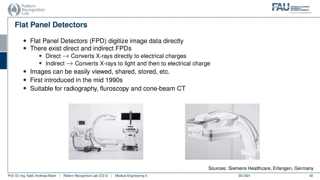
Flat panels are also cool because you can also operate them close to a magnetic field. So this is very nice. What’s then again a bit of a challenge is if you want to operate an X-ray source actually within a strong magnetic field. Imagine if you have a rotating anode and you would do that inside of a strong magnetic field. Well, that’s actually how an electronic brake works. So it’s not such a clever idea to work with rotating anodes and x resources in general within an MR scanner. But actually, it can be done but for example, you want to choose a static and or design in this case. Now if we have these flat panels they are cool because they don’t need this additional acceleration. So they are flat and one reason why they became really popular is that they are more effective so they have better efficiency and they are also small there. There are much smaller and if you think about flat panel displays and those vacuum tube-based kind of CRT displays that have been used prior to flat panels. A major advantage is that you have much more space on your desk right and this is the same also in medicine. Also, one major reason why flat panels became very popular is that you don’t need this huge bucket and you can get much closer to the patient and get much better angulations and cooler images of your patient. So this is a key reason why flat panels have been actually introduced and they were first very popular in the interventional field. Still, it took some time to convince medical doctors of this new technology because they suddenly had different zoom functionalities. So there were no continuous zoom functions available anymore because of the missing electron optics and yeah the contrast to noise ratio was better with this one. So you had a more crispy clear image. So finally if people could then be convinced to introduce this technology. But to be honest this was introduced in the mid-1990s and I think I’ve seen image intensifiers still around in the 2005-2009 years. So they have been used in the hospitals. So maybe if you go to a hospital you might still encounter the image intensifiers that we’ve seen on the previous slides. So this is the well new stuff if you say the mid-1990s. That’s not so new stuff actually but finally, this technology actually went to replace most of the image intensifiers. 

There are different types. There is the direct conversion and the indirect conversion. So the direct conversion converts the X-rays directly into electrons. So you do that in a single step and then there is this indirect conversion where you have a Scintillator material.

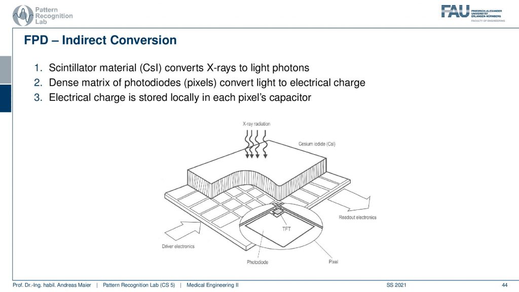
 Then you still have photodiodes and they then detect the light and the light is then converted into electrical charge. And you can see here that you then typically have this kind of TFT arrays here that are being used to then measure the actual information that is contained in the pixel. 

So the readout is very similar for the two and there are these thin foil transistors that are being used but let’s not talk about all of the details of the actual data readout.

Let’s rather look at the different sources of noise along the path.

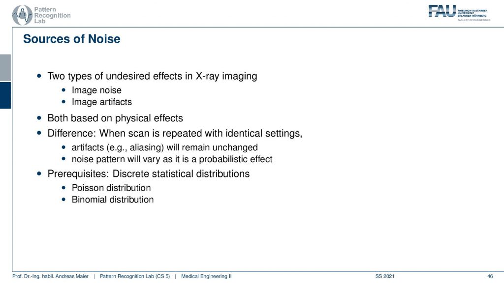
You see that we have different types of noise happening here. So there are the undesired effects of course and the one key thing is noise and the other one is image artifacts. Both of them are determined by physical effects. And if we understand the physics we can understand how they propagate and which properties they have. So this is very important. Also if you want to compensate for them you have to understand the physics and if you understand the physics you can build a model that is able to reduce this effect of the undesired artifact that shows up. Now in order to understand what we do on the next couple of slides, we want to look into noise distributions and therefore we have to understand discrete statistical distributions in particular the Poisson distribution and the binomial distribution. So these two are key if you want to understand the processes of noise generation along the X-ray path.

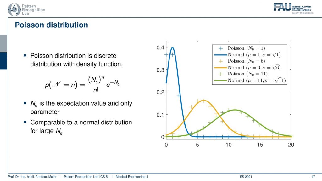
Now let’s start with the Poisson distribution. For the Poisson distribution, you see that this is the formula for how we can calculate it. So you have some (N₀)ⁿ to the power of n and then this exponential term here which is also dependent on N₀ and you have the factorial of n here. Now if you have different instances for N₀ which essentially determines the shape of the distribution and is the expectation value and the only parameter of our Poisson distribution. So if I have a low kind of expected value here then you see that I get an observation here or here. So this is the discrete sampling. There is also a comparison here where we have the normal distribution that is approximating this Poisson distribution and it’s shaped in this form. So actually this is a discrete distribution and this is actually why we shouldn’t call it density but it’s a probability mass function because we only observe it in discrete values. So you see that the Poisson distribution here is only at discrete points and they need to be discrete numbers. If I create a density from this I have to take the normal distribution as an approximation. So you see here that this is the normal distribution that approximates best the specific Poisson distribution. You see also that there is a mismatch between the two and if you have relatively large and zero if you choose this value to be high then you get something that is very close to a gaussian distribution. Still, it’s different and in particular for the low counts. The difference to the gaussian is rather large and therefore you want to have at least one. Let’s say a hundred in terms of n such that you can actually switch to a gaussian distribution. Also, one key problem here is that you have this factorial of n in here and this makes it also rather expensive to compute. So if you want to have large numbers of n then the factorial will be very expensive to evaluate. This then also brings up an estimation formula that kind of brings us close to whatever we are going to expect. So this is the Poisson distribution. We’ve seen the shape and let’s have a look at an example. 

So how would we use the Poisson distribution? So let’s say we have a local shop and this local shop writes down the number of customers per day for one year. So now we have discrete observations and it’s the number of customers. It could be also a number of Photons right and this is exactly why we want to use this later on because we’ll use it for Photon statistics. Now the average number of customers per day N₀ is 15. So we can compute that and estimate N₀ and then we know what number of customers we can expect. Now with the Poisson distribution, we can now determine the likelihood that tomorrow we will have 20 customers in the shop. We computed setting N to 20 and yeah you can do the math. This is our N₀ this is 15 and then we have the 20 that we have to plugin here and you see already that we have to compute the factorial of 20 here. If we evaluate this term we see that it’s about 0.0418 and this means that the probability for observing 20 customers tomorrow is 4.18. So this is how you use the Poisson distribution. 

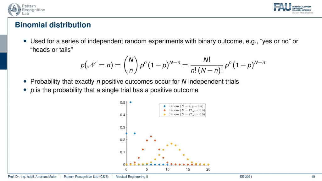
Let’s go to the other distribution that is of relevance for understanding the noise properties. And this is the binomial distribution. The binomial distribution is now using this N over n term here and that’s the binomial coefficient and with that, we can then essentially estimate the outcome of repeated experiments where we toss for example a coin. So this is with binary outcome. So yes/no or, heads/tails and with the binomial distribution, we can approximate the sequence of yes or, no experiments. You can already guess that we want to use that for the interaction of the photons with matter. So we essentially have the question will the photon be absorbed or not. So that’s the yes/no question and this means that we end up in binomial distributions. So again the binomial distribution can be modeled and describe the probability that exactly N positive outcomes occur for n independent trials and p is then the probability that a single trial has a positive outcome. So you see here different shapes for our n and our p and you see that they get this particular form. Obviously, if I choose the p to be 0.5 so this is essentially a Laplace contour and then you see that the more often I toss the coin the more it smears our distribution. If I throw fewer coins I essentially get distributions of this shape and if I have very few coins I only have these observations here. So this is again a probability mass function and it’s not a density but let’s keep it to the formulation here on the slide. It’s a bit inaccurate but we can still live with that. We will be pickier in the latter set of slides. Now let’s also look at an example and what can we compute with the binomial distribution. Let’s toss a coin 30 times and compute the probability that we turn up 20 times heads.

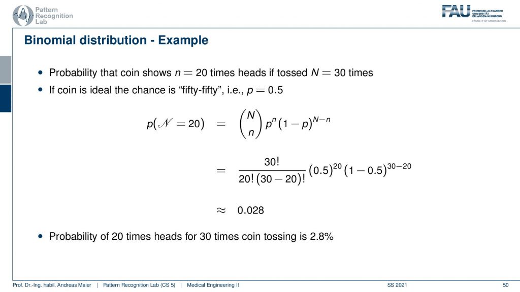
Now let’s say this is an ideal coin. So we have a 50 50 chance and then we can plug in our numbers use the binomial coefficient. So here goes the probability of the number of heads and here the number of tails see you have to plug it in at the right positions and then you can evaluate this entire expression and what you get is 0.028. This means that the likelihood of observing 20 times heads when tossing a coin 30 times. So you exactly observed 20 times heads is 2.8%. Obviously, if you want to know that the occurrence of more than 20 times then you have to add up essentially 20 times 21 times, and so on. So you have to compute the integral if you want to more than 20 times heads. But if you want to know exactly 20 times heads then you can compute this probability here. So this is the other distribution or probability mass function that we want to use in our experiments or in our X-ray physics. 

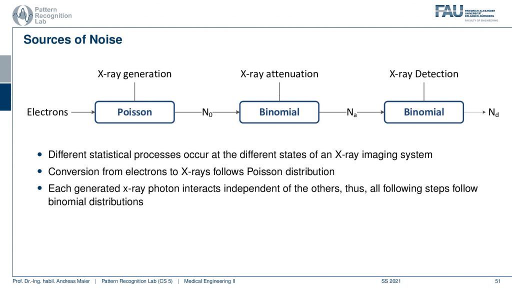
What we can see here on this slide is that the generation like the customers entering our shop follows a Poisson distribution. Then the attenuation that this stuff gets absorbed is binomial and also the X-ray detection is binomial because it’s essentially describing probabilities of being absorbed. So we can see now that if we have a noise process we have some electrons starting the process. Then we kind of have the generation and the attenuation and they are all described by these different probability mass functions. So if we now have a final observation in a pixel how it will be distributed? 

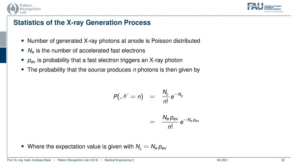
This is interesting because if we follow the steps in the propagation then we can figure out that if we have an X-ray generation we can compute essentially the probabilities of observing a certain number of photons exactly here with our Poisson distribution. So now if we want to observe n photons then this probability is given here. Obviously, this is dependent on the expected value of the number of photons that it’s going to be produced. 

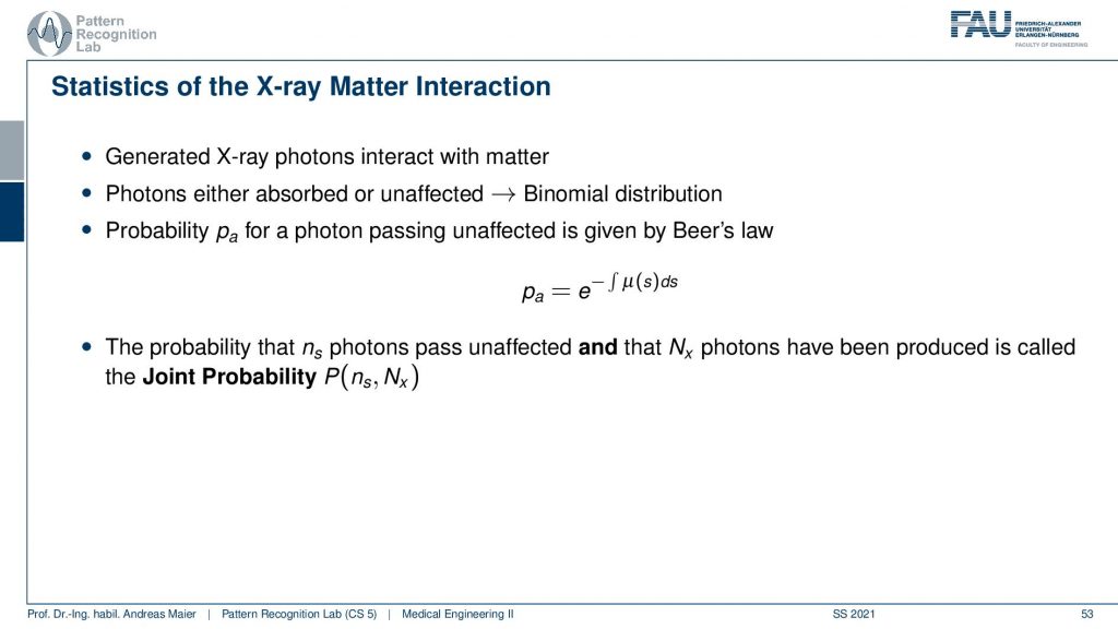
So we can then use this and then send it through the entire process. What now happens is that the Poisson distribution essentially follows into binomial distribution and we have the whole interaction. Now the interesting thing is if we now propagate everything statistically through the entire process, then we essentially come up with Beer-Lambert’s law. So if you just derive everything from probability theory you can see that the probability for a photon to be passing unaffectedly through the entire object can be determined by this e to the power of this integral here. Now you see that what I already mentioned in the first video when we talked about the actual interaction with matter that this e to the power minus the integral this is a probability. It tells you the probability of a photon to be observed. Now you can also understand that if I have some intensity zero or some this is essentially proportional to the number of photons. The number of photons times this probability gives you exactly the observed photons. So this is essentially the mean value over the entire stochastical process that is given by Lambert-Beer’s law. So that’s pretty cool that you can propagate only from probabilities to this entire process and in the end, Lambert-Beer’s law falls out. So that’s cool!

Now if we know that and by the way also when we observe the final signal on the detector, we will see that if you have a binomial process on a Poisson process it will still be a Poisson process. 

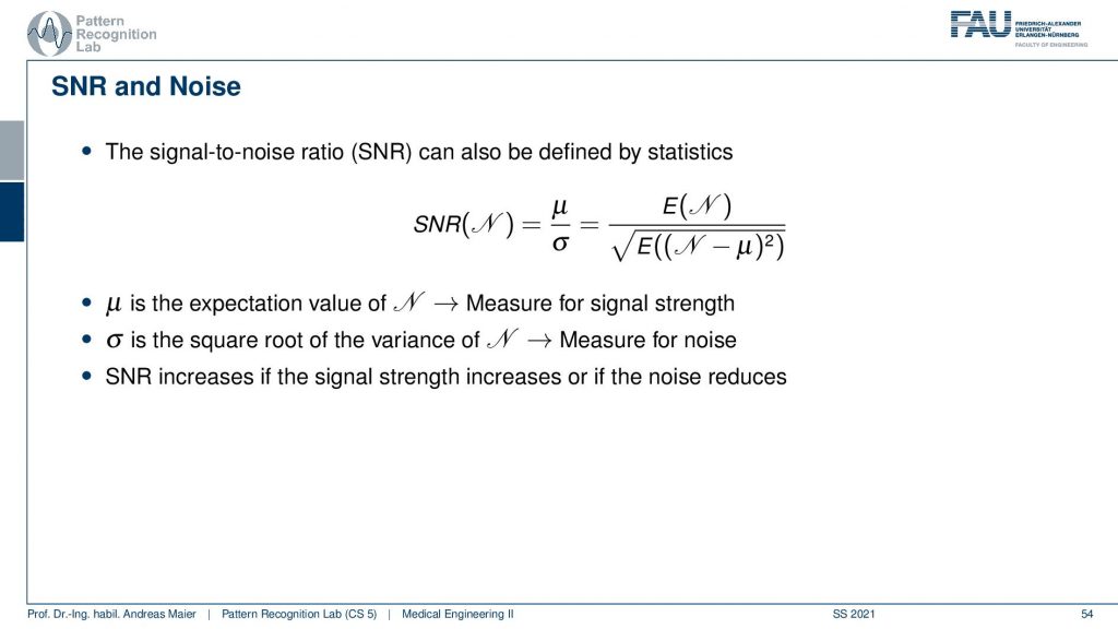
And this then allows us to determine the so-called signal-to-noise ratio. So the signal-to-noise ratio as we define it here is the expected signal divided by the standard deviation of the signal. The standard deviation of the signal is essentially the square root of n and it’s a measure for the noise and μ is the expected value and it’s a measure for the signal strength. So the SNR increases if the signal strength increases or the noise reduces. Now, this is interesting because we know the probability density function here or the probability mass function.

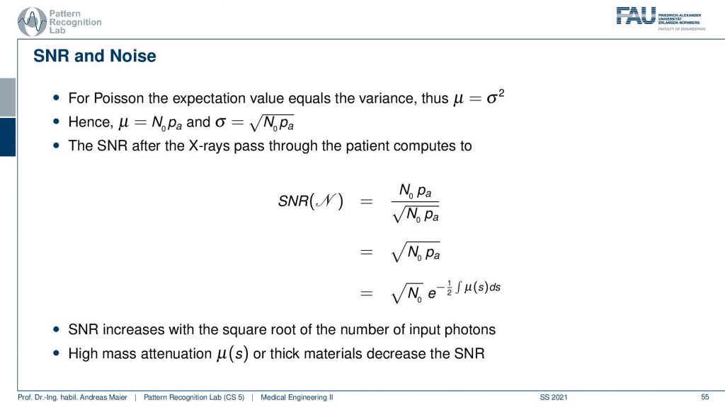
And now we can plug in our Poisson distribution and we know that in the Poisson distribution we will have a mean value of N₀ times p_a. So this is what we expect to observe on the detector. We also know that the noise is given by the square root of the mean value. So in every Poisson process, the standard deviation is simply the square root of the mean value. This is cool because they’re both dependent on N₀ times p_a which means that we can directly write up the signal-to-noise ratio. So we put in the signal. This is the expected value. This is the square root of the expected volume. You divide by it so you just end up with the square root of the expected value and now you can still take out this probability. Here you still have to add the 1/2 because you’re pulling it out of the square root and then you see that the signal-to-noise ratio is essentially dependent on the square root of the number of photons that you’re using and the actual absorption along the path. So these are the two components that drive the noise. So the thicker the object is the higher the absorption is along the path, the noise level will increase. Also N₀, the number of photons at the source determines the noise process. This by the way also means that in every pixel you have a different noise level. So the thicker the object at this particular pixel, the difference is then also observed in the noise level. So that’s also something to think about.

Well let’s continue and what we still want to talk about are actual applications of X-rays and most of you already know the applications of X-rays. 

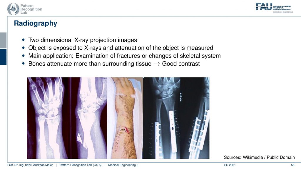
So there’s radiography where we essentially create transmission images to diagnose the bones or, implants. After implantation, you want to check whether everything is still in place or whether you have a broken bone. This is a very clear application of X-rays, in particular in the extremities you can use them very well because in your arm and legs there is essentially only the bone marrow that can develop cancer. Most of the other tissues and arms and necks are not very sensitive to radiation. So there it’s pretty safe to use it. It’s different in the inner organs. So there you have to be a little more careful. If you are caring about radiation and X-ray dose there is a wonderful plot by cake cd where you can figure out how much those are emitted from different kinds of emission sources. So it’s not just medical X-rays. So medical X-rays and CT play only a minor role but there’s of course also radiation emitted in nuclear power plants and in if there is an accident in nuclear power plants. Then you can see many many orders of magnitude higher in terms of radiation. But still, it gives you a feeling of how dangerous actually the technology is and how you can relate a chest X-ray image to a CT and to the Fukushima incident. So there are very very different levels of radiation introduced there. So I will link that in the description.

Now the next application is fluoroscopy. We already talked about fluoroscopy. These are essentially X-ray movies and there you also want to be sure that you have a low frame rate because the more images you make the more X-ray those you actually inflict. This is mainly used in interventional applications. So very traditional application is fluoroscopy in minimally invasive interventions. 

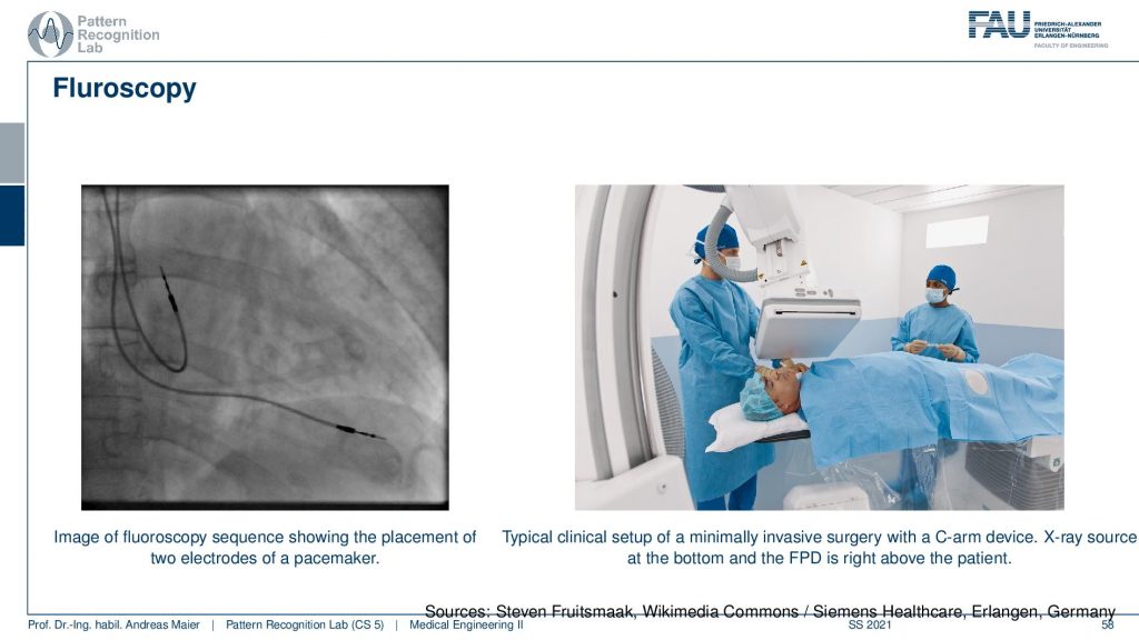
And here you see an application where there’s actually a catheter being set into the heart. So there’s typically standing if you have the hard vessels they narrow down and if you want to improve the flow in the heart you put in the stand. We’ve seen that already in the introduction and this can then help us to recover very quickly from stenosis and bad blood flow in the heart. This can be restored with this kind of X-ray-guided procedure where you take a wire and then go into the hard vessels and open them again. Stroke is also a very typical application for this.

There is this wonderful technique that is called digital subtraction Angiography and this uses an additional contrast agent. So you take some material that has a high X-ray absorption in particular iodine is suited for this and iodine causes a lot of absorption. So you inject it into the blood and then you take two X-ray shots. So you take one with contrast agent and one without and then you subtract the two and this is digital subtraction imaging and we’ve already seen that also in the introduction. 

So the principle is that you take two shots one mask and one film image and then you overlay them and subtract them and we’ve already seen this in the introduction. 

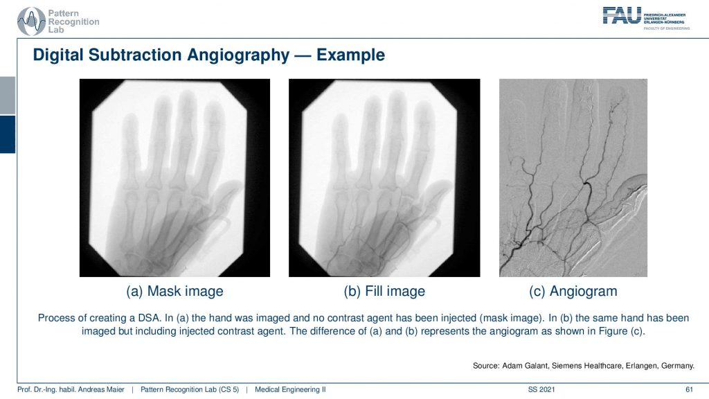
So this is how it looks like. On the left-hand side, you see the mask image and then this is the fill image and if you compare the two you barely see any difference right. You have to look very closely to see the vessels here but if you subtract them then you get this wonderful angiogram. You see the vessels well and you see even vessels appearing here in the thumb that you couldn’t see in the previous image. So that’s a very very popular technique and I can tell you this is an invention that brought the field ahead quite a bit. But all you need to do is subtract two images. Just take two images and subtract them. You can find a pattern on that. So that’s a marvelous invention and had a huge clinical impact. Well, this already brings us to the end of the set of slides.

So if you have questions you can put them in the comments or you can also send them by email or on our online learning platform.

We also have a reference for the last three videos and this is the chapter by Martin Berger in our lecture notes. So I recommend having a look at it because there are also very interesting stories about Röntgen in history and so on. So please have a look at our textbook as well. I hope you enjoyed this video and you found this quite useful that we talked a bit about the actual detection and how it’s being converted into something that we can measure and then display as an image. We also talked about the different noise that is happening from the X-ray generation that has a Poisson distribution and then the whole absorption processes always have binomial distributions and with that, we can model essentially the entire noise along the path. In the end, this forms a Poisson distribution. With the Poisson distribution, we’ve seen that the mean value of our statistical process is the Lambert-Beer law. So you can interpret also the entire imaging chain as a sequence of probabilistic events on photon level and you can reconstruct the entire Lambert-Beer law from that. So that’s pretty cool! Isn’t it? 

Well, I hope you enjoyed this video. If you found some things not so easy to follow please also tell us. You can of course leave some comments. You can engage in the deep learning platform and I’m very much looking forward to seeing you in the next video. Bye-bye!!

If you liked this post, you can find more essays here, more educational material on Machine Learning here, or have a look at our Deep Learning Lecture. I would also appreciate a follow on YouTube, Twitter, Facebook, or LinkedIn in case you want to be informed about more essays, videos, and research in the future. This article is released under the Creative Commons 4.0 Attribution License and can be reprinted and modified if referenced. If you are interested in generating transcripts from video lectures try AutoBlog

References   

1. Maier, A., Steidl, S., Christlein, V., Hornegger, J. Medical Imaging Systems – An Introductory Guide, Springer, Cham, 2018, ISBN 978-3-319-96520-8, Open Access at Springer Link
2. KXCD Dose Chart https://xkcd.com/radiation/

Video References

1. Lumbar Transforaminal Epidural Neurogram https://youtu.be/CTyIu-EGby8
2. Trans-Femoral Valve Fluoroscopy https://youtu.be/5J6NxFhI6ns
3. Preclinical Cardiac Angiography https://youtu.be/zQq9lrN5Ex8

Category: Lecture Notes in Medical Engineering