Computed Tomography – Concept

These are the lecture notes for FAU’s YouTube Lecture “Medical Engineering“. This is a full transcript of the lecture video & matching slides. We hope, you enjoy this as much as the videos. Of course, this transcript was created with deep learning techniques largely automatically and only minor manual modifications were performed. Try it yourself! If you spot mistakes, please let us know!

Welcome back everybody to Medical Engineering. Today I want to take the opportunity to start looking into the technique of Computed tomography. So the idea here is that we can use X-rays to create shadow images of the patient and we’ve already seen that this essentially are sums along the ray. Now we want to reconstruct the virtual slice images like virtually chopping the patient into slices and then look inside the patient such that we can improve diagnosis. So looking forward to exploring computed tomography with you guys. 

So computed tomography is a rather modern technique. So it has been implemented first in the 70s. Since I think 1974 it is a technology that then went on to the clinic. But actually, the history is much longer and I want to show you also the mathematical principles behind this. So we’ve already seen that for the imaging itself we very heavily relied on MRI imaging and on the Fourier transform which is about 250 years old. The theory for forming the images from computed tomography was only discovered in 1917. So you see that the technology in terms of math is only about 100 years old. So let’s see what I have for you. 

So we start with the motivation and brief history.

Now the computed tomography approach is one of the most important technologies in medical imaging because it allows us to look inside the body and really spatially resolve parts of the inner organs and so on. We can also use contrast agents such that we can also make specific structures better visible and it is the first volumetric modality that has been discovered over history. We already talked about MR. So this point is not entirely true but we are essentially following the mathematical development here. So in other courses about medical engineering, you probably talked first about CT and then about MRI. But I found it much more intuitive to start with MRI because the mathematical principles of imaging are much older and therefore we will need some of them when we want to understand the principles of CT. You will see that actually in this in the next videos why we already need the knowledge about the Fourier transform to understand what’s happening here on CT. 

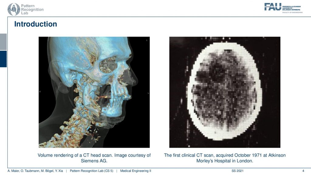
Now CT is a great modality to image heart tissues like the head bone or, the spine. It is the first modality that was able to look inside the skull. On the left-hand side, you see a modern image a reconstruction that shows very nicely the bones and this is a volume rendering. On the right-hand side, you see the first CT image that has ever been created in a clinical environment. You see that this is a very interesting image because you can now look inside of the head. This image is actually 80 by 80 pixels and so you have 80 pixels here and 80 pixels here. So it’s a rather low-resolution image. But it shows us the X-ray absorption coefficients at every point inside of the head. We can look inside of the head without actually having it cut open. Imagine you would cut through the skull at this point that would be a pretty invasive kind of surgery and now we can look inside the head and discover things. What’s really exciting here is you see there’s a lot of artifacts. So you see that the skull here has these white shadows that appear so they’re not really present but what’s much more exciting about this image is the position where you can see this dark shadow. So there is some area in the brain that has a very different contrast in the surrounding tissue. Here you can see that this can diagnose the cause of certain diseases and we don’t have to open the skull. We can figure out things about the patient before we have to do an intervention. It also contributed a lot to understanding the brain structures and the neural anatomy in the early days. So really a wonderful technology and of course people got very excited about the kind of images that have been generated here. This is also one of the reasons why CT imaging has been awarded a Nobel prize.

Now let’s think about what we can do with that. 

So typically x-rays are used to acquire 2-D projection images and in the 2-D projection image, everything is superimposed. So everything along the ray is just projected into a single pixel. So we only see shadows of the imaged object. But we would like to look inside and I have an example here.

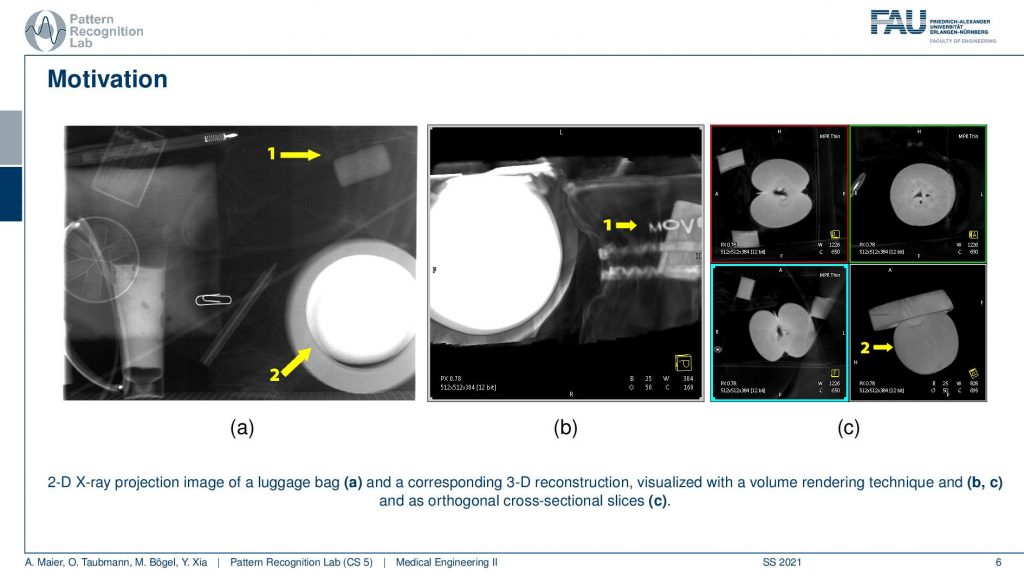
This example shows a couple of images and one thing that you can do for example is here on the left-hand side you see the X-ray projection and it’s very difficult to actually discover anything. What you can now do is you can essentially cut planes through our object here. So you can actually cut a plane and then look at this plane. Then you can discover for example that there is a very thin bag here and you can even read some of the letters that have been presented here. So you can make things visible that have not been visible before. You can also see in the second example here this is object number two. Object number two is this guy here. You can barely recognize it if you have a volume rendering, it looks like this. Now you can see if I choose the slices appropriately through different regions here, you could probably think that the green one is slicing in this direction right. So this is nice along here and then you have the blue. Let’s say the blue could be for example a slice that runs here through the object and then there is still the red one. So the red one could be a slice that runs like this through the object. So this would be the red plane and this would be the blue plane. So you can fully volumetrically discover the object and while on the image it may be hard to actually figure out what is shown. Then you see here when I slice through this object you can see this is a kind of fruit and it’s probably an apple. So this way we can understand what’s happening inside of the object and of course, you recognize images like this one because this very much looks like an apple when you cut it through. So we know how to cut apples and we’ve seen cut apples and this way we don’t even have to touch the apple. So we just have it here inside of a bag or inside of a box and we can still uncover the contents of the box. So that’s a really exciting and cool technology and with this, we can now use this for diagnosis.

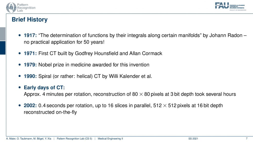
Let’s shortly discuss the history of CT. You see it goes back to 1917 because in that year Johan Radon discovered the mathematical principles of how to invert the line integrals. So this is a paper actually published in the German language and this paper here actually has not been used for 50 years. Only in 1971, the first CT scanner was built that then used essentially those principles in order to construct slice images. The inventors and creators of CT were Godfrey Hounsfield and Allan Cormack and both of them then, later on, went on to win the Nobel prize. So this was awarded in 1979 and the next breakthrough you could say that was determined here is in 1919. This is the Spiral or, rather helical CT acquisition that was discovered by professor Willi Kalendar and he was a professor of FAU. So he was teaching at our institute. He retired a couple of years ago. But he is the inventor of the helical city and helical CT was the breakthrough technology that essentially got rid of the problem that you have to determine certain slices. But with helical CT you can really acquire continuously entire volumes. So really cool technologies and you see that in the early days of CT you had like four minutes per rotation. You had reconstructions of 80 x 80 pixels and 3-bit depth and the reconstruction took several hours. Now in 2002 you already had 0.4 seconds per rotation. So we actually have to rotate about the object in order to acquire the image. We could reconstruct 16 slices in parallel in 512 x 512 pixels at 16 bits depth resolution. So this could be reconstructed already on the fly. 

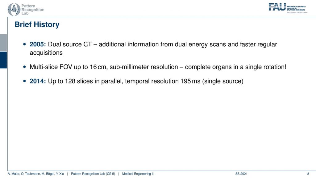
There have been some further improvements in 2005. The first dual-source CT emerged and this is a CT gantry that has two sources and two detectors. With this, we can acquire multiple energies at the same time. So, you remember when we discussed X-rays that we have different X-ray energies in different spectra. If I measure two of the energies then I can also start thinking about material decomposition and really create quantitative numbers from the scanning. Then there was also multiple slice field of view scanners with a field of view of up to 16 centimeters that can be acquired in a single spin. This is also quite a bit of a breakthrough. In 2014 up to 128 slices in parallel at a temporal resolution of approximately 200 milliseconds could be determined with a single source. If you use it on a dual-source system you can even double this acquisition speed as in the dual-source scanners you have two sources and two detectors you can actually acquire at a much faster rate and you get below 100 milliseconds in terms of acquisition time today. So this is enough to create volumetric movies of the heart and in contrast to gated techniques that then rely on a cyclic or periodic heart motion, this kind of technology can also be used to image asynchronous movement i.e. non-periodic heartbeats. Obviously, if your heart is sick it might happen that it’s not moving in a way that you would expect it. So it could have some non-periodic motion and this can all be acquired in a single go on a modern-day CT scanner. So there are really cool CT scanners out there that allow doing so.

Here is one image of such a CT scanner. Now in this scanner, you can see that you actually have a gantry. So this is the gantry. So the source and the detector are moving here about the patient. So we need to rotate about the patient to generate the x-ray image. Here you can see that this kind of scanner also allows a tilt. So you see that the entire gantry can be moved back and this is now at an angle to the floor. So it doesn’t stand upright but it can be moved down and the idea behind that is that you scan the patient at a different angle and this is particularly interesting if the patient faces pointing towards the top. You can scan the entire brain with these kinds of tilted slices without having to scan through the eyes and that’s very efficient in terms of those. So this is a reason why you can actually tilt those gantries in order to avoid scanning through organs that are very sensitive to those like the eye. So this is one modern-day scanner and obviously, these scanners are now also much more dose efficient, image quality has improved a lot. It’s also quite interesting to see an open view of such a scanner because they rotate very very quickly in modern-day scanners up to four times per second a complete rotation. So this is a technology that allows us to scan very quickly in high resolution. If you want to scan a full body so from head to toe you can do that on such a machine in approximately 10 seconds. So here you also need fast patient beds in order to be able to move the patient through the scanner quickly enough. So this is typically then also used in emergencies where you only want to spend very little time on the diagnostics and the acquisition and of course, this is also very useful if you have motion breathing and so on. Then the scan can be performed very quickly. It’s still a really important technology in the clinic.

Now we want to try to understand the mathematical principles behind this.

A key principle is the Radon Transform that was discovered in 1917 and the so-called Fourier slice theorem because this is the main principle that allows us to build fast reconstruction algorithms today. So what will we cover?

Well, the Radon transform is essentially the acquisition. So it’s the mathematical principle of how the image is acquired and it’s an equation that builds on the line integrals and we’ve already seen that the x-rays are nothing else than acquiring sums along with the rays of their line integrals. Now the inverse Radon transform allows reconstructing from the projection images the original slice images or, the patient information. The Fourier slice theorem is a key result that has been identified by Radon which allows us to reconstruct very quickly and we will try to demonstrate all of this mainly in a visual manner. So we’ll use some equations but now if you understood what the 2-D Fourier transform is then you should be able to follow these ideas without having to go through all the equations. Obviously, we also have all the equations in the textbook. So if you want to understand the math in a more detailed fashion then you can also go back to the textbook. So what we then want to cover in the next video is the core idea of the important reconstruction algorithm. So today’s video will mainly look into mathematics and the guiding principles. How we can actually reconstruct images.

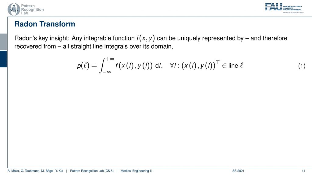
So we’ve seen in the previous video what we actually can observe on our detector and source is this relation that I equals to the original intensity times this e to the minus the integral and this is essentially f(x) along the direction of x. So this is the ray penetrating the object. Remember this guy? So this was our patient. This is our source and this is the detector. So you see that this is the detector. Then this is the source and what we are actually interested in is our patient. So our patient is already anonymized right. This is our patient. He’s called f(x). Now we want to solve this and we can do that really quickly because we can simply take this equation and rearrange it such that we divide it by I₀ so, I divided by I₀. Then we take the natural logarithm and minus and then we see that the only thing that remains here is this integral over f(x) along with the ray dx. Yeah, so this is x in my example here is x. So this is a 1-D coordinate system where this is x and our patient is f(x). Now, this only describes a single ray. So that’s stupid. So let’s rewrite this and we are now using the integral above. So we are changing the notation. So p is now the projection. This is the solved line integral that we had as the integral over f(x)dx on the previous one. So this is our p(l) and you see now that I’m using l and l is the line and now we want to have multiple lines. So we essentially determine this line as a line running through a 2-D space and now this 2-D space has components x and y and we change the notation here. So maybe we should call this x’ or something like this. Let’s call it x’. If this is x’ then we could also have an arbitrary wave running through here and this would be x’. Now at every point along this line, we integrate, and obviously now our f(x) is this entire slice here and maybe this is the slice that we want to reconstruct right. So what we do is we now essentially have to access a 2-D function. We have to access the 2-D function at the points where we are actually intersecting. So we need more of them right. We want to intersect everything here along this line. So in this direction, it’s just a 1-D integral. So you could say if I compute the integral along this x ‘ then we’re in this formulation here. But instead, I can also say okay I integrate over this entire plane here. I integrate over the entire green section here and now I have to rewrite this because this is the 1-D integral. So this is the purple element here. So I’m integrating along the line but obviously, I have to figure out where I’m actually in this 2-D image. So I’m only accessing the red points here. So these were the red points and these are the coordinates of the red points here and I do that for all elements that are essentially on this line. Obviously, I can also rewrite this. I can essentially integrate over the entire domain here. I can integrate into a double integral over this entire section and then I will add everything up but I’m only doing it at the position where the line actually is. This is an alternative formulation that we’ll find extremely useful. 

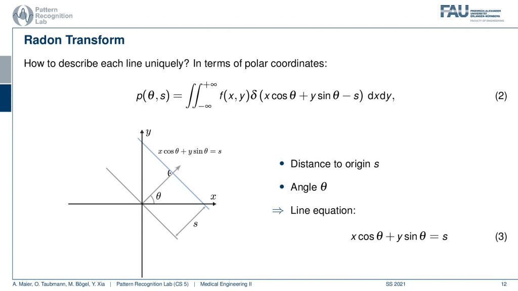
So we will see that nowhere this is a double integration. So this is integration from minus to plus infinity along dxdy. So you see this is our dxdy plane and now we add a δ function and the δ function is a function that is zero everywhere except at zero. And if you look very closely here this is exactly our line. This is the line here and if the condition xcosθ plus ysinθ minus s equals zero then we are exactly on this line.  The δ function is going to be 0 if we are not on the line and it’s going to be 1 for the line. So if you’re on the line it’s going to be 1 and everywhere else it’s going to be 0. Now you can already see if I do this mathematical trick what then happens is that although I’m summing over this entire plane here I’m multiplying with 0 everywhere except for all the points on this line. You see also that this line equation here this xcosθ plus ysinθ equals to zero shows up exactly here in this argument because it’s simply subtracting x. So this is an equals zero condition. So if I subtract s here I get exactly the condition that we have here. So now you can understand this equation that it is essentially a kind of less efficient implementation of how to compute this line integral because effectively it only computes the sum over all the elements of the line. But I’m actually iterating with a double for loop over the entire plane. Typically you don’t want to implement the line integrals like this in code because you have essentially a complexity of N² if this is N. But integrating only along this line here would give us a complexity of only N. Still mathematically both formulations are exactly equivalent. 

So why do we do this? 

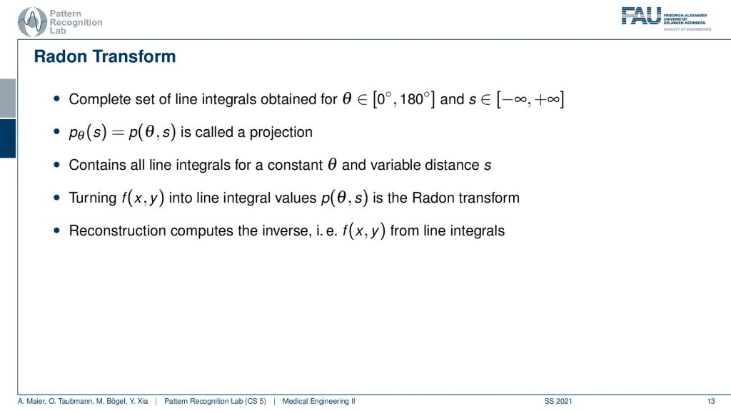
Well, we can see now that if we rotate 180 degrees all around the object we get all the set of line integrals. So you can imagine this in the following way if you actually start acquiring an object and the object is of course in the center of rotation and now I start acquiring here. I’m collecting all of those line integrals here. Then I rotate let’s say by 90 degrees then I’m gathering all the line integrals here. At 180 degrees my detector is here and I start just collecting exactly the same line integrals again but just in the opposite direction. So you can see now that the 180 degrees and the 0-degree projection are exactly the same except that they’re flipped. So I’m not creating any new knowledge by rotating more than 180 degrees which is the reason why we only define our rotation angle between 0 and 180 degrees. Obviously, we have to integrate over the entire line from minus to plus infinity. We assume also that our objects are on a compact set which means that in practice our object only lives in a space somewhere inside of our coordinate system. This way we can omit the integration from plus to minus infinity because we only need to know the bounds of the object and then we only integrate within the object. So this is the key idea that we want to do and the reconstruction problem is now given all of the projections how can I get back to this kind of object. Here that’s the key problem of image reconstruction.

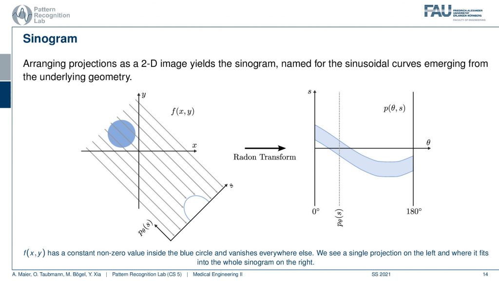
We can write this up a little more formally or use an example because this leads to the so-called sinogram. So the sinogram is the sequence of all projections. You see that our f(x) lives in this 2-D space and now we can convert this into a different domain. So we convert this into a different domain and this is now also a 2-D space but it is the 2-D space in s and θ because these are all the projections right all the projections that I gathered. So all of those guys here now become lines in this two-dimensional space. The rotation direction is actually the second direction here. So this is this guy here and this is called a sinogram. It’s mainly called a sinogram because if you have an object here, it will be projected onto a sinusoidal wave. So if you think about rotating about this point and thinking where this circle will be projected to then you can figure out that it will start moving on sinusoidal waves in this kind of projective space. So this is the sinogram. That’s the key observation by Radon. This sinogram here is enough to describe the entire object. So if we know the sinogram then we can reconstruct the object and if we know the object by projection or simulation you can reconstruct the entire sinogram. So they’re both essentially equivalent and you’ve already seen this kind of relation with the Fourier transform. With the Fourier transform if you know the 2-D Fourier transform like an MR, we can reconstruct the object. If we know the object we can reconstruct the 2-D Fourier space. So again this is a kind of transform between you could say two basis representations. Yet the projection on the line integrals is not really an orthogonal basis like in the Fourier transform case but it has redundancies. So because the points essentially contribute multiple times to the same observation. So this is something you have to keep in the back of your mind but this is the transform into the projection space. Now the inverse random transform is the idea of how to reconstruct from your projective space back to the image space or volume space. That’s the key problem that we want to solve.

So this brings us to the so-called Fourier slice theorem

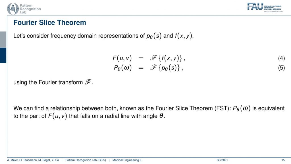
The Fourier slice theorem now introduces an additional Fourier space here. You’ve seen previously that this is the Fourier transform of our object space and our sinogram space. What the Fourier transform says, in this case, helps us to understand the identity between two relationships. So now I’m introducing a Fourier space for the actual object. So this is a Fourier space of the object and let’s take a different color. So let’s say this is our Fourier space. So these are all Fourier values and we are transforming using the Fourier transform here. Now what the Fourier slice theorem tells us is that there is a relation between those two Fourier spaces. There are identities between the Fourier space of the slice image and the full space of the projection image. They are related and that is the key observation of the Fourier slice theorem that also allows us first of all to guarantee the completeness of the actual acquisition. It also tells us how we can reconstruct. So the Fourier slice theorem says that if you have a projection at a certain angle θ, the line that coincides through the center of Fourier space with the exact same angle has identical coefficients. So the 2-D and this 1-D Fourier space have coefficients that are identical. So we can show this in a small image. 

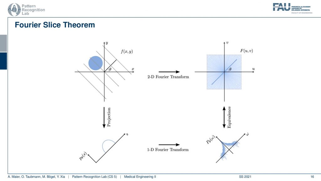
So we already know the above relation. So this is our object space. You remember this guy. This is our sinogram space and now we introduce the Fourier space here on the right-hand side. Now what we are saying is that the Fourier transform of the 1-D projection, so the Fourier transform of this guy. So this is a single projection image and I’m taking a 1-D Fourier transform. Then, of course, I get a 1-D series of coefficients and these are identical to the coefficients in a 2-D Fourier space along this line and it’s the line that runs through the origin here. So we can say okay if we would know all of the coefficients here, if we could sample everything here then we would be able to use it to the inverse Fourier transform to get back to the image. And obviously, if I know the image then I can use a 2-D Fourier transform to go back to the Fourier coefficients. Now the problem is I do not observe the entire image. So I don’t know this guy here. So I don’t know this guy and the only thing I know is these guys. Now the key idea is that I can essentially do the projection. Then I have the projections, I go to Fourier space. Then I have 1-D coefficients and now I know that all of those 1-D coefficients run through the center. Now if you see that I rotate by 180 degrees our lines then I essentially have the star-like figure that samples all of the coefficients in this 2-D space. Then I can use an inverse 2-D Fourier transform and get back to our image. Sounds a bit complicated because I have to do the projection. I have to do a 1-D Fourier transform, an inverse Fourier transform, and this kind of rebinding here from these lines over the kind of radial transform there. So this is a bit complicated but it generally allows us to get back to our original image. So that’s cool and Radon showed this in 1917. So this is his main achievement. If you know this then you can also design a reconstruction formula and the reconstruction formula is still known as the Radon Inverse.

This is a bit difficult to follow and I want to show you an intuition why this is actually the case. 

So we remember this figure of the 2-D Fourier space. So you know that if I want to get essentially this point here, I need to take the original object image and multiply it with this plane wave. Here I take the entire object image. So you remember in our case it was this kind of circle here. So I multiply this point-wise sum everything up and then I get this point and if I want to get this point I take our 2-D object. You remember it looks like this. I multiply the two images, this plane wave and the object, sum everything up and write it in here. If I want to get this point here I need my 2-D image. I multiply it at every point, sum everything up and I get exactly this coefficient and the same is also true here. So if I want to get this particular coefficient then I need to multiply at every point, sum this up and I get this coefficient. So this is how I would get the 2-D Fourier space if I knew the object. Now I don’t know the object. So I have to be more clever in order to get it and the idea that we now have is that we want to use projections.

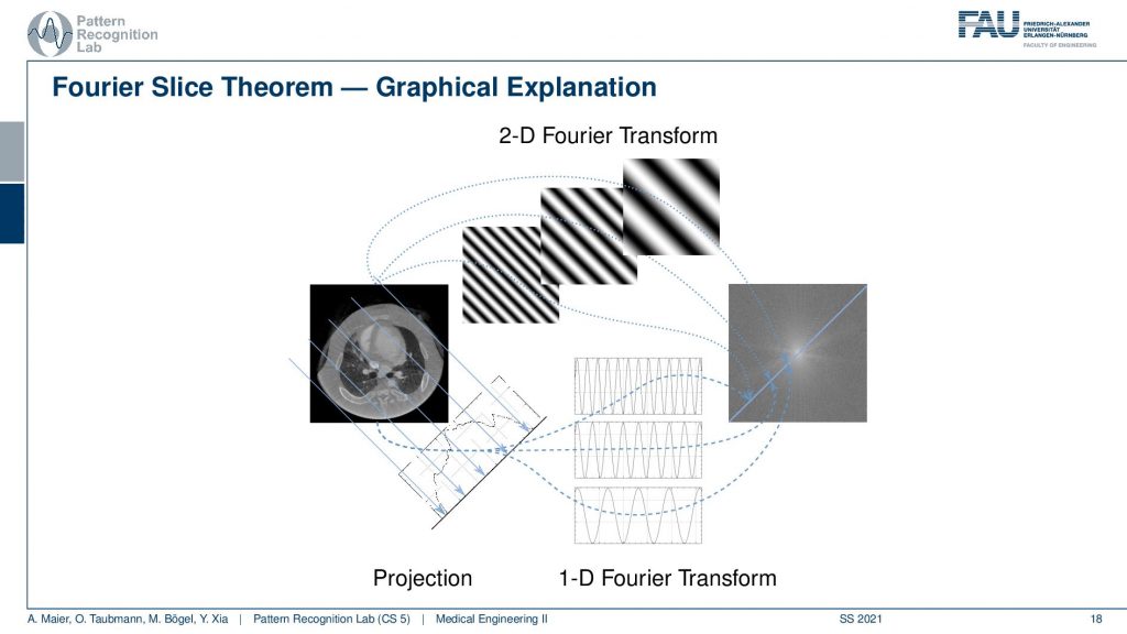
I have this kind of image and I hope it helps. You understand what’s actually happening when we’re computing a parallel projection. What we are actually doing is we are summing all of the coefficients along with the rays. So this is our 2-D space right and then summing all of the coefficients along with these rays right. And if I do so I get my projection image. Now if I compute the 1-D Fourier transform what I’m actually doing is I take all these sine waves here. I multiply them point by point so it overlays essentially my projection image here. I do a pointwise multiplication and sum everything up and if I do so then I get exactly this coefficient here. If I use a different frequency now I’m using a slightly higher frequency and now I overlay the projection image multiplied them pointwise and this will give me exactly this coefficient. Now I take a very high frequency like this one and I overlay the projection image, do a point-wise multiplication, sum everything up and I get exactly this point here. So this is the path that allows us to determine the individual Fourier coefficients along our line here. So this is the Fourier space and we have just found all of the coefficients along this particular line here. So this is the line that came from the projections and it has exactly the same angle θ as you would have. So if I take the angle here this is also going to be θ. So you see that this is one path to compute those coefficients. Now obviously I could also take the path of the 2-D Fourier transform. Here you remember I need those plane waves and all of those plane waves have the same angle. So they all have the same orientation. The only thing that changes is the distance between the hills and the valleys right. So it’s just a different frequency in the direction that is perpendicular to the projection direction. 

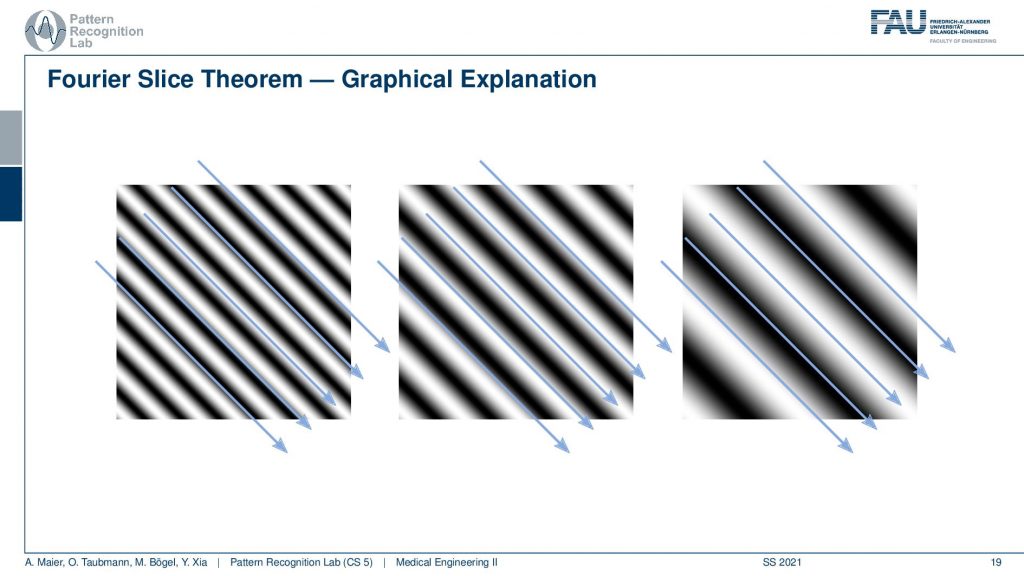
So you can see if I look at those plane waves here what they are actually computing is they compute an integration along this path and a Fourier transform along this path. This is what’s happening with this plane wave. It computes a Fourier transform in the one direction and an integration in the other direction. You can see that very nicely here that essentially if we overlay the projection operation you see that everything is simply summed up along this direction because in the very end we sum up over everything in this plane. If I follow this direction you see I have a kind of sinusoid in the one direction and I have a kind of integration into the other direction. You see this is the sinusoidal wave. So that’s pretty nice! Because now I have essentially discovered that I have two different paths that compute exactly the same coefficients. So I have the paths with the 2-D Fourier transform that exactly determine those coefficients and I have the path with the 1-D Fourier transform that exactly determine the coefficients. So I hope this helps you to understand why this Fourier slice theorem actually holds and this is a graphical representation of Fourier’s nice theorem. 

So this is how you can compute the Fourier slice theorem and how you can link the Fourier space of the projected image and the Fourier space of the actual size image with each other. That’s the key discovery and this tells us that from all of the projection images we are able to reconstruct the actual image. Now what I didn’t tell you so far is actually how to compute the reconstructed image. I just showed you the path there. There’s actually a couple of methods that allow doing so and we will discuss them in the next video. So now you’ve understood that the data that we are acquiring is sufficient. In the next video, you will understand how to actually design an algorithm that solves this system of linear equations very efficiently. So I hope you enjoyed this video and found it kind of instructive and I’m very much looking forward to seeing you in the next video. Bye-bye!!

If you liked this post, you can find more essays here, more educational material on Machine Learning here, or have a look at our Deep Learning Lecture. I would also appreciate a follow on YouTube, Twitter, Facebook, or LinkedIn in case you want to be informed about more essays, videos, and research in the future. This article is released under the Creative Commons 4.0 Attribution License and can be reprinted and modified if referenced. If you are interested in generating transcripts from video lectures try AutoBlog

References   

1. Maier, A., Steidl, S., Christlein, V., Hornegger, J. Medical Imaging Systems – An Introductory Guide, Springer, Cham, 2018, ISBN 978-3-319-96520-8, Open Access at Springer Link

Video References

1. Randy Dickerson – Syngo Via VB20 Cinematic Rendering https://youtu.be/I12PMiX5h3E
2. Book CT – https://youtu.be/q67HOVpLub0
3. Radiographer Films Inside of a CT scanner spinning at full speed https://youtu.be/pLajmU4TQuI

Category: Lecture Notes in Medical Engineering