Computed Tomography – Reconstruction

These are the lecture notes for FAU’s YouTube Lecture “Medical Engineering“. This is a full transcript of the lecture video & matching slides. We hope, you enjoy this as much as the videos. Of course, this transcript was created with deep learning techniques largely automatically and only minor manual modifications were performed. Try it yourself! If you spot mistakes, please let us know!

Welcome back to Medical Engineering. Today we want to continue our journey through the mathematics and algorithms of computed tomography. What we want to do today is we want to discover the different algorithms that are used to reconstruct the images. So I’m very much looking forward to looking into the reconstruction algorithms of computed tomography.

So here we see how we want to proceed with the reconstruction algorithms and today’s topics are essentially the main reconstruction families. There is the analytic reconstruction and the algebraic reconstruction and there’s also a couple of changes in acquisition geometry that allow us to make much faster acquisitions. So these are the main topics that we want to discuss in the video today. 

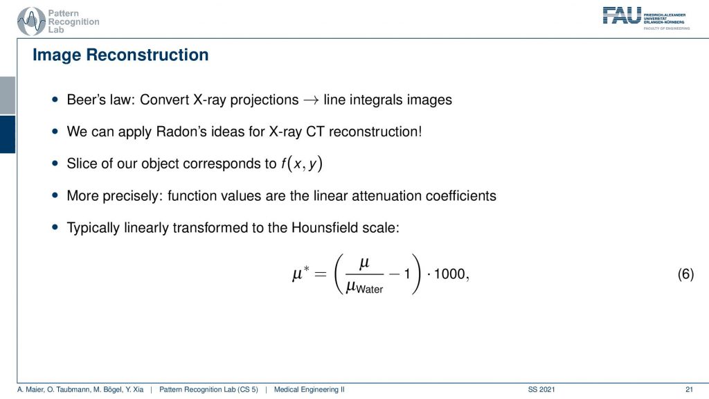
Now let’s go ahead and have a look at the reconstruction problem. One key problem that we have is that the X-ray projections. They essentially form line integrals and we understood how we can essentially get the original information but what we still haven’t discussed is that these μ are dependent on the X-ray energy. So somehow we want to be able to create standardized values. This is why in reconstruction theory we have introduced so-called Hounsfield values. The Hounsfield values now standardize the absorption coefficient that we know is energy-dependent and they are divided by the absorption coefficient of water minus one. So if you have water this would be exactly one, you subtract one and then you multiply with 1000 and the unit is then given as Houndsfield units (HU). Now the Hounsfield units have the property that they’re exactly zero for water and they’re -1000 for air. So these are essentially the two points air or no density would be zero and water would be exactly one after the scaling. This means that we have a kind of standardization for water and of course water is the most important material inside of the human body. This is why this kind of scaling has been chosen. 

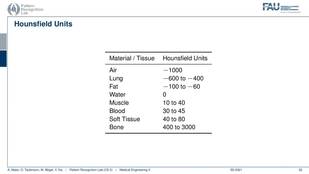
This comes with a couple of interesting effects. So first of all the standardization only holds for air with -1000 and water with zero. For all the other tissues, you see that we have different kinds of value ranges. For the lung -600 to -400, for fat -100 to -60. Then we have Hounsfield values that are higher than zero and for bone, the range is between 400 and 3000. Now, why do we have these ranges? First of all, the human tissues are of course variable. So not every human is built in the same way and we can easily standardize for water and air but for human tissues, it’s more difficult. Second, depending on the choice of your acceleration voltage and the x-ray acquisition you will have a different non-linear effect on the actual Hounsfield units. So the standardization only holds for water and air and all the other Hounsfield units that are generated from this. They are dependent on the actual acceleration voltage of the imaging process. So you get a different contrast if you image at 120 kV or 80 kV the images will appear differently and this is also what then gives rise to this range of Hounsfield units.

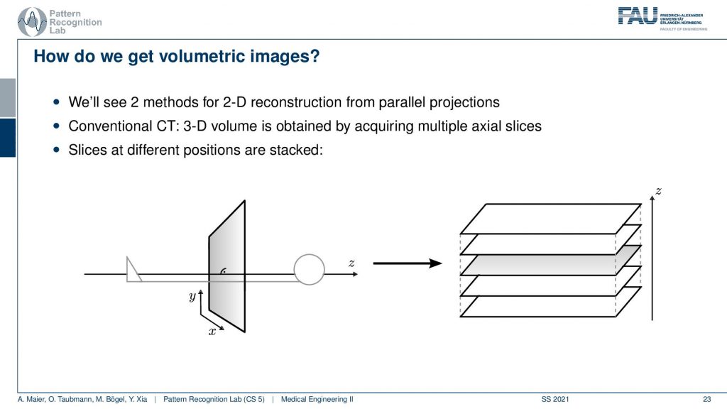
Now the next thing is how can we get volumetric images and yeah you see here we had a kind of object. We don’t want just a single slice but we only understand how to reconstruct one slice here but obviously, you can stack this. Yeah so I can just repeat the acquisition and this is how the first scanner by Hounsfield and Cormack was working. It had a line element. So it was only acquiring a single line here and it had a detector that was even more difficult because it had just a single source element and then also a single detector element. What they did is they translated them to build an entire acquisition. So this was a parallel beam acquisition like this one here and they needed to shift here in order to construct the image. Then if you want to construct the next slice you have to shift essentially into the z-direction. So you now essentially shift this is the acquisition plane. So this is x-y that we’ve seen previously and now I take it and shift the entire thing into the z-direction in order to get multiple of those slices. So that’s the key idea of how we can get to volumetric images. Now you also might understand why it’s a cool technology to have a helical scan because then we can do the acquisition in a continuous mode. Here we have to stop, acquire, shift, acquire, and so on. So this takes a long time. So this is also the reason why the original scans took so long. With the modern systems, we can be much faster because we discovered the continuous effects of the different motions involved here. Also, we are using very different detector technology

Now how would we then derive a reconstruction algorithm?

We can use the Fourier slice theorem to derive an analytic reconstruction method. So the key idea is that we start with the inverse Fourier transform of our object. We’ve already seen that the object can be given as f(x) and if we had the entire Fourier space then the inverse Fourier transform would solve the entire issue. Now if we want to do that then we need the Fourier transform of the slice and we will get the reconstructed slice. So what we do in order to get an efficient solution is we use polar coordinates where we have the angle θ in here. This is very important because we’re acquiring on a polar coordinate system right because we’re rotating the detector about the patient and we are dependent on this angle θ here. This can be done by substituting u with these polar representations here. If you want to do so this is also something that you learn in mathematics that requires a correction with a factor that is computed from the so-called jacobian matrix. The Jacobian matrix is the derivative with respect to the different variables and then you take the determinant of this matrix. In our case, it boils down to the absolute value of ω. So now we know that we have to multiply in addition with the absolute value of ω. 

This means that our Fourier transform in the polar coordinate system can simply be expressed as the Fourier transform and polar coordinate system and then multiplied with this absolute value of ω and still the remaining Fourier transform. Here is essentially a Fourier transform. Differences are now that we integrate over the angle here which means that we have integration from 0 to π and the other variable is still a continuous variable. So this is from minus infinity to plus infinity along the frequency variable ω. 

So if we stick to this then we can now use the Fourier slice theorem. So we know that the Fourier transform of the projection image is identical to the polar version of our 2D Fourier transform. So we simply replace it and we can now do this change here. The two are identical and now we have a reconstruction formula that has essentially the projections on the right-hand side and the reconstructed image here on the left-hand side. We somehow have to compute the Fourier transform of the projection. There we can also simply take the definition of the Fourier transform and plug it in.

So you see here that the Fourier transform here is found in a 1d version. You see this guy here. This is a 1D Fourier transform along exactly the direction in which also our detector is pointing. This means that we can convert this back into the original domain. So we can save some time and here you see then that we have the Fourier transform of the absolute value of ω appearing here and we also have the original projection data appearing here. So we know that multiplication in frequency space is a convolution in the spatial domain. This then brings us to the so-called filtered back-projection algorithm the more or less the Radon inverse. This is done by filtering with an appropriate kernel h(s) of the projection data. And then we just have a sum over all of the projection angles that give us the reconstructed point. So these steps to actually perform the reconstruction are filtering and a back projection. With those two steps, you can solve the reconstruction problem. That’s cool because of the filtering we can do in Fourier space. So we have a nlogn operation and the back projection is just a single sum. So it has a complexity of n. So this is a very efficient method to solve the reconstruction problem. Yeah, so this is the filter that’s introduced here. So in order to do that we have to determine this filter and the filter also has a very nice property. 

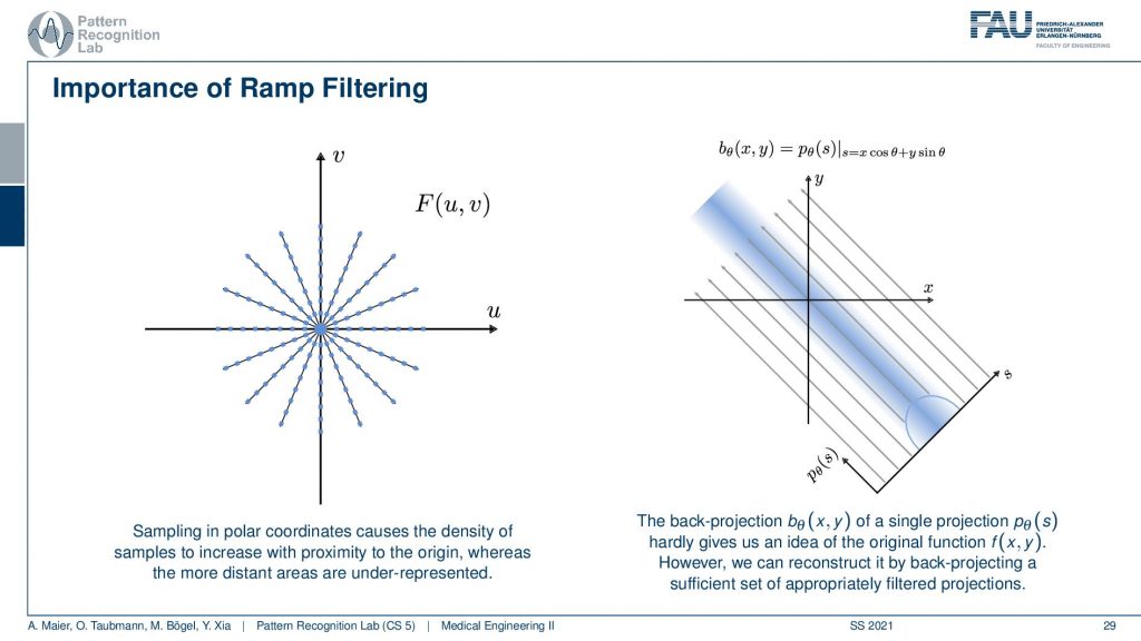
So you can see that we’ve seen that the absolute value is being used here and we have already seen that in the previous video. If we sample on this polar space you see that the density is much higher in the center. The density of observation is much higher in the center than in the outskirts. What we are doing essentially is we take one of those lines here and multiply it with the absolute value of ω and the absolute value of ω looks like a ramp. You can see that the sampling pattern essentially goes down in density towards the outside. So we need to ramp up the values on the outside and in the center in a continuous space, actually, in the perfect center, you would infinitely times observe the zero frequency. This is why we are waiting with zero in this ramp filter in the zero frequency. Obviously, this is not true if you’re going to discrete space and you have to care about this position in the ramp filter a lot when you’re implementing this in a discrete version. This kind of filter is then applied to our projection image. You convolve with the Fourier transform of this ramp filter and then you back project. So that’s already how you would reconstruct.

Then we still have to talk a bit about this kind of filter.

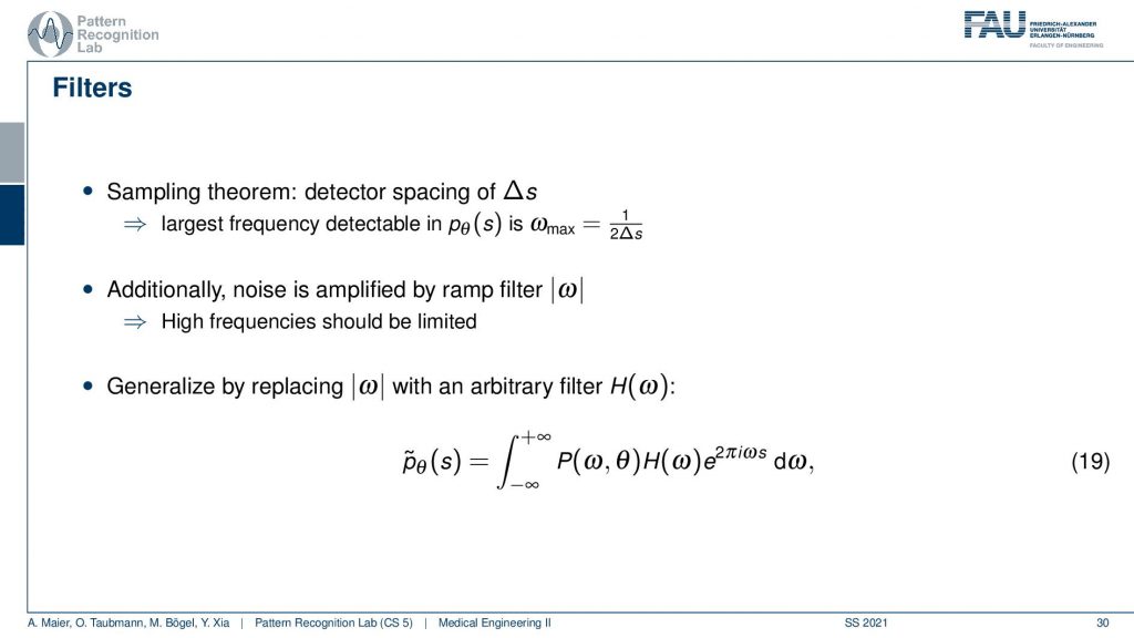
We need to actually cut off certain frequencies because we know that our detector has only finite element sizes. So there’s a detector spacing and this has a finite size of ∆s. So there is a maximum frequency of 1 over 2∆s and this one has to be applied to our ram filter. So the ram filter doesn’t look like the one that I’ve drawn previously which just goes all the way to infinity. But instead, you have a cut-off frequency here and here and the filter that we’re actually using has this kind of shape. So then we can actually generalize an arbitrary filter here because we may want to incorporate also other kinds of operations. So you see that this is a high pass filter. So it will be very prone to noise and when we are filtering anyway we can also incorporate other filtering operations such as noise reduction and a smoothing operation. This then results in alternate filters that have an additional roll-off. So if you also want to punish high frequencies you might then get a filter that looks like this one. So you have a rolling off towards the end of the Fourier space because you want to punish the high frequencies in order to avoid excessive noise. But you still want to keep the low frequencies because you want to reconstruct the object correctly. 

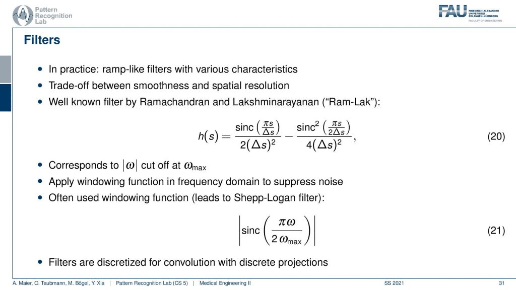
Well, this can then be done also in a mathematical sense. The cut-off version of our ram filter has a representation in the spatial domain that you find here with this equation. We’re not deriving it here. You can look into the textbook we derived it actually there. There’s a very elegant solution that allows you to derive this in only three or four steps. So that’s actually quite efficient and oftentimes. This is then also weighted with one of those cut-off filters which is essentially a sink that is in on top multiplied into the signal. This then leads to the so-called Shepp-Logan filter which is similar to what I’ve just shown to you. 

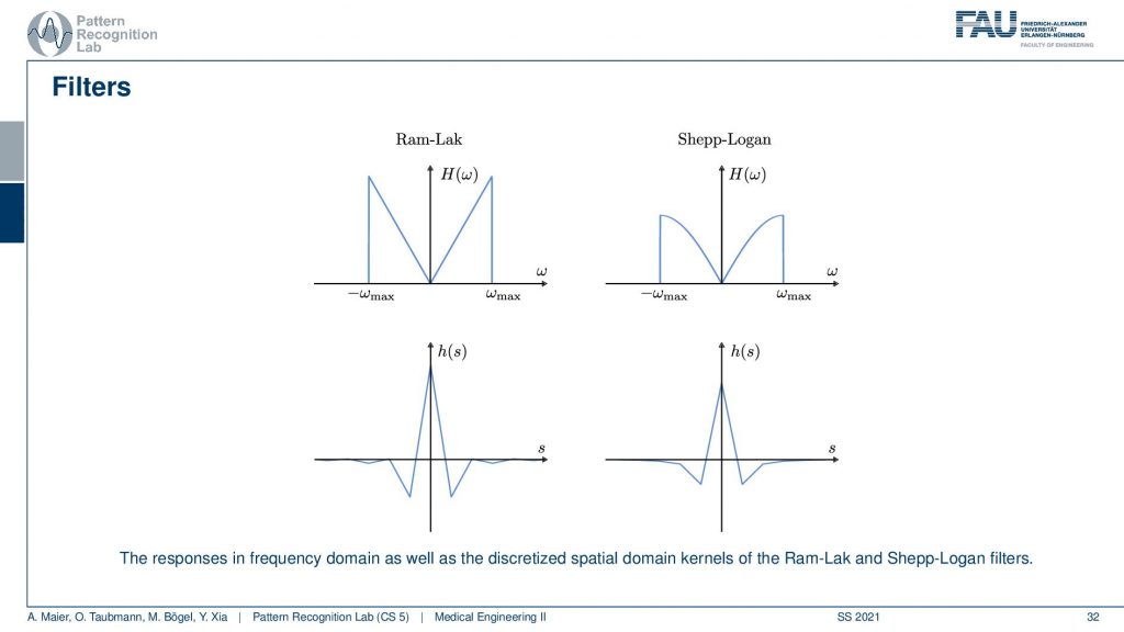
I also have graphs in case you don’t want to follow my actual drawings here. So you see that in the previous version I had a roll-off that was much stronger that was going down here and here. This is I think the cosine filter that I’m drawing here in red. But you see that we kind of punish the very high frequencies and the original ram lag goes up all to the very boundary and then just cuts down to zero. So these are different solutions for this filter and with this filter, I can then get the final filtered back-projection algorithm that is a convolution.

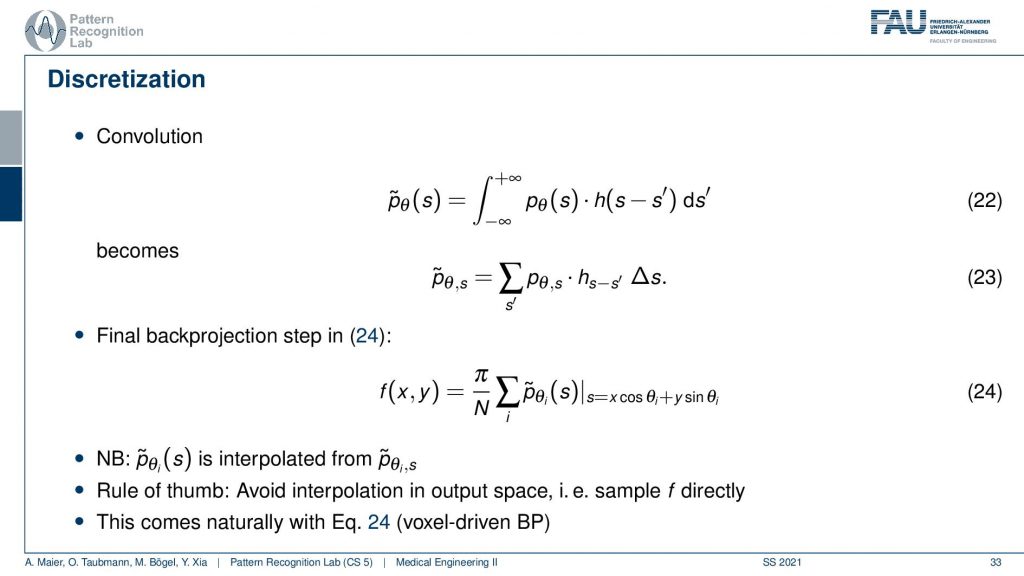
Now the convolution is actually on a discrete projection. This is what we’re actually computing and now you see the integral in discrete space. They just become sums. So it’s a sum with our actual filter and the projection image. I sum it up and this gives me this filtered projection image and the filtered projection image is then without any further ado. We don’t have to go to Fourier space anymore because we’ve seen it essentially cancel out. We immediately plug it in to compute our slice image. And this is done by the so-called back projection and what’s happening here is that I’m computing this s essentially as the footprint under the projection. So if you have your image here, this is what you want to reconstruct. This is our f(x), the position and now what I do is I’m essentially projecting this in a parallel manner on all of our projectors. This then gives me the element here and the element here. So these are all 90-degree angles because we are operating in a parallel beam projection. So this is already the filtered back-projection algorithm. So you implement the filtering, you implement this sum along all of the footpoints that you can compute with this kind of equation and then you get the reconstruction of one point. Then you iterate over all of the points in the plane and this will give you the entire reconstructed image very efficient method and still very commonly used in CT reconstruction. 

There is an alternative to this and the alternative to this is the so-called algebraic reconstruction.

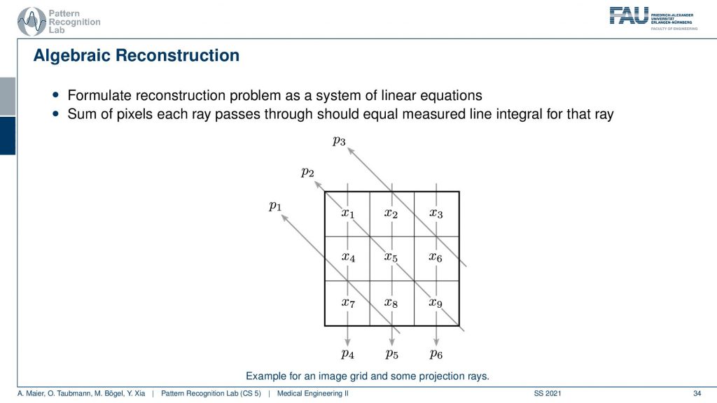
The algebraic reconstruction is essentially the solution that emerges if you discretize first and then solve. The filter back projection is considering everything in the continuous domain. And then you discretize towards the very end. Now if I want to consider the reconstruction problem discretely, I could also describe the CT problem as a set of unknowns and some projection rays. I have my projection rays here as p₁, p_2, and p₃. This means then that for example for this p_3, I can simply write it up as the sum of x₂ plus some weight. Let’s call it α₁. Then we also have so x₂ is considered x₆ and x₃ right. So we have x₃ and some α₂ and we have x₆ multiplied to some let’s say α₃. So what we see is essentially the volume. This is the volume or, the slice image. Then I can find an equation for every projection. So what I can do now is I can write this up as a long kind of vector. So for all our projection rays I can find this in a vector and write this up as p₁, p₂ and p_3, and so on. I can write this in the long vector and I can also write our entire volume so x₁, x_2, and so on. I can also write this in a long vector and then you see that I essentially have a matrix in here. This matrix now has line-wise these coefficients. So we can write up this entire reconstruction problem as a vector p that is given as a matrix A times a vector x. That’s the entire reconstruction problem from a discrete point of view. So it’s a complete matrix equation just one matrix and you can write up the entire forward projection and then the inverse of this matrix would simply be the solution. 

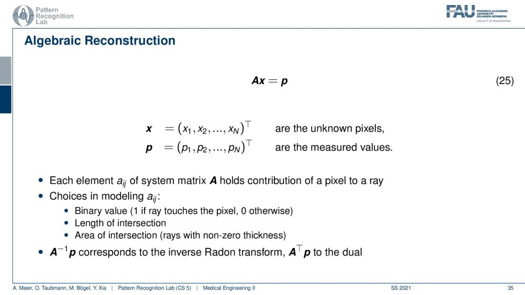
Well you see that we can write this now as an equation and now each element a_ij has essentially the geometric information and it essentially tells you how strongly the voxel is related to this particular point in the projection. Most of the entries of a are actually zero. Because if it’s not touching the ray, if the voxel is not touching the ray it has zero contribution to that particular pixel. So most entries are zero and you can then do different models. So you could say I can model a_jby a value of 1 if the ray touches the ray and 0 otherwise. I can compute the length of the intersection or, I could even compute the area of intersection to determine those weights and you see the more effort I put into modeling this the more realistic my forward projector gets. But there are many different choices that I can simply model as this matrix A. So now what we want to do is we want to compute A inverse and this actually is nothing else than the Radon inverse that we’ve seen before. So this is a very interesting observation but we can also solve it discretely. Now a key problem with this A is that it’s really huge. So if you have a volume that is 512x512x512 and you have projection images that are 512×5 12 pixels and you have 512 projection images. Then you can instantiate a matrix that is 512 to the power 3 times 512 to the power 3. If you want to save this matrix in memory, just the geometry you will need 65,000 terabytes of memory in floating-point precision. So that’s not a good way of actually implementing this and this then gives rise to the so-called iterative reconstruction approaches. 

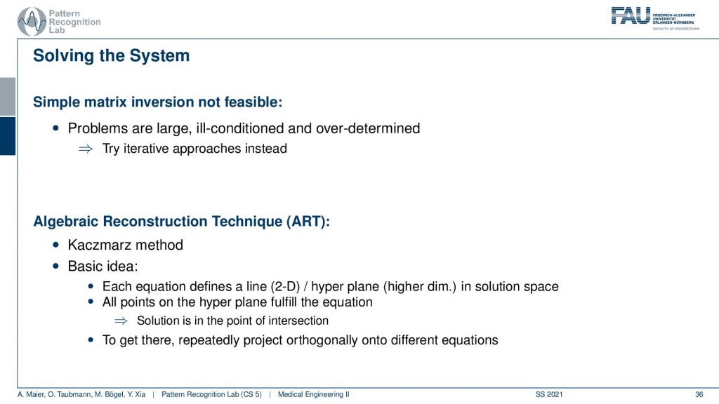
So the simple solution is not feasible. This is really large. It’s ill-conditioned, it’s overdetermined and it doesn’t really work. So let’s try to solve it iteratively and this is where the so-called algebraic reconstruction technique art comes into play. It’s also called the Kaczmarz method and the basic idea is that you try to iteratively approximate the ideal solution of all the line equations. Once you found a new solution for one of the line equations you project the solution onto the next line. So we have essentially only point and plane intersections in order to compute the new update. And we can successively do that. Now how does this work?

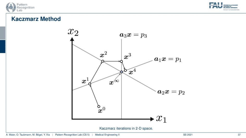
Well, I have a very nice image here. So you can see that we start with some initial point x⁰ and then we have a first projection. This is our first projection and we now compute a parallel projection of this point onto our first projection and we get an update. Let’s first have a look at what’s actually shown in the space. So you see here that this is the value x₁ and this is the value x₂. So what I’m showing you here is a volume that only has two unknowns. This has the unknown x₁ and the unknown x₂ and the entire space. So this is not the reconstruction space. So these are all possible configurations of this volume that you see in this space. Now I start with random initialization. So you start with some x⁰. So this could be some initialization that brings us here. And then I may have observed some projection p₁ here and this is then the update such that the observation that we got along this line integral now matches the current state of the volume. Now I can also do another projection. So I’m doing the projection p₂ and now p₂ is a different linear combination of those two variables. And now I can use this again to create an updated configuration of the volume. Then I have a third kind of projection that is p₃ and maybe p₃ runs in this direction for the volume. So you see here that p₃ is essentially only associated with the variable x₁. Now you can see that we can use this information again that we construct an update and we update again and we update again and again. Then we iterate until convergence and we exactly end up at the intersection of those three lines. So this is the Kaczmarz method. 

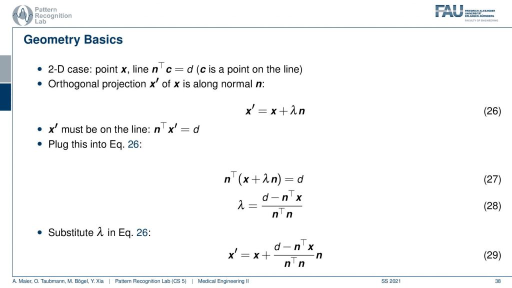
Now we can also write this up as equations and you’ll figure out that this is rather easy to construct because we know that the new observation x prime has to be on some projection of the old configuration. You see this is our original configuration and this is the normal vector of our projection line. So we essentially have to determine this λ here in order to find our updated point x’. We also know that we have a line equation for our observation. So this is d but it was it’s one of those three and this is one of those equations. We see here that the new projection of x’ needs to fulfill this equation. That’s the orthogonal projection. So now we see that this has actually x’ also appearing here. So we can take this definition and plug it in. This gives us this new equation. Then we can multiply in the n^T and subtract the n^T. So here we have the n transpose going in here and going in here. Then we take the left-hand term here and subtract it and we take the right-hand term and divide by this n^Tn is an inner product between two vectors and this is just a scalar value. So this is how we can then solve for our λ and then we can use λ and plug it in back in here. This gives us then the new configuration down here where we have the update x’ equals to x plus this fraction here times the normal vector. So it’s essentially a step length that we have to follow in order to get the intersection with the new point. So this is all just line intersections and orthogonal projections. Now I iterate this over all of our set of the projected pixels and finally, I’ll find the point of convergence. This is also a way that allows us to find a solution without having to instantiate the entire huge matrix A that had this many nonzero elements. 

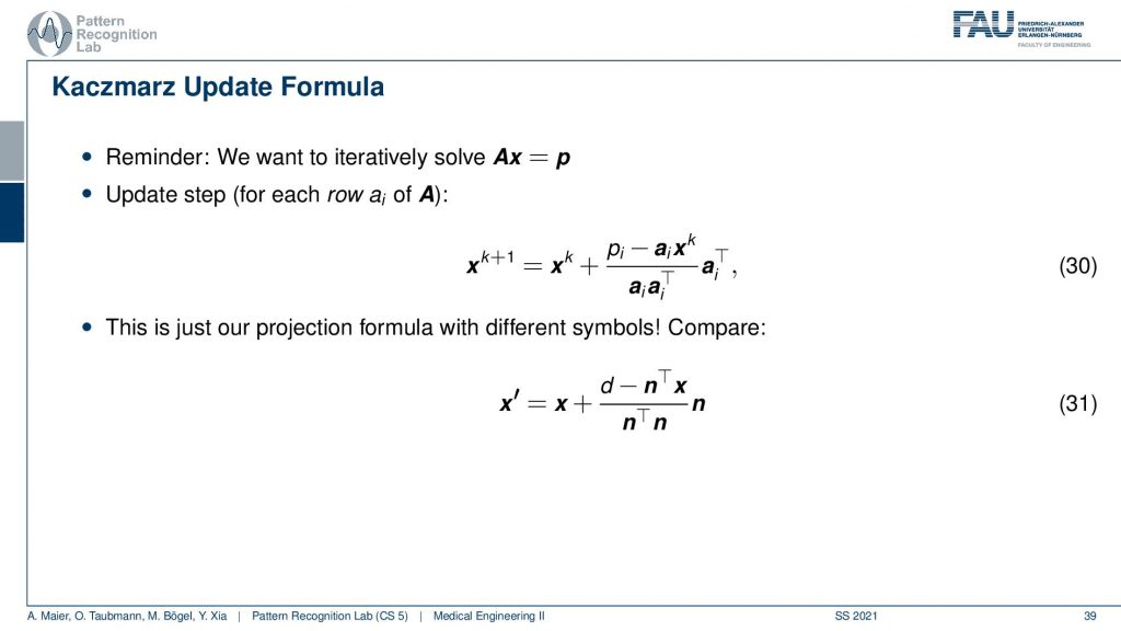
So this yields then the Kaczmarz update formula and yeah you do that over the iterations. You see I now replace this with the iteration index and further you can now see that the ns are equal to the elements of this matrix. So you see that this is essentially a very similar configuration and we derive this entirely geometrically. 

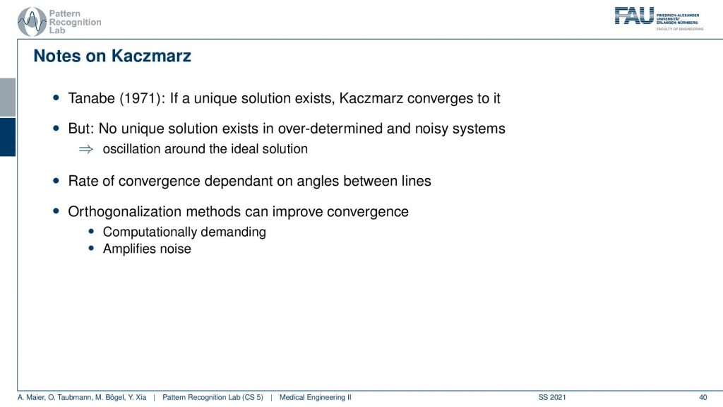
Some notes on the Kaczmarz method. There is a unique solution if there is no noise present. So if there is no disturbance is present it will iterate and just find this unique solution. So, that’s pretty cool! but if there’s noise present then there is oscillation. It won’t converge in noisy conditions and you have to abort at some point. Another thing is that the rate of conversions is dependent on the angle between the lines and then there’s also tricks how to rearrange the system of equations such that the matrix lines essentially are orthogonal and this brings up quite a bit of convergent speed if you manipulate the system of equations and this is some kind of trick that can be used to solve it more quickly. 

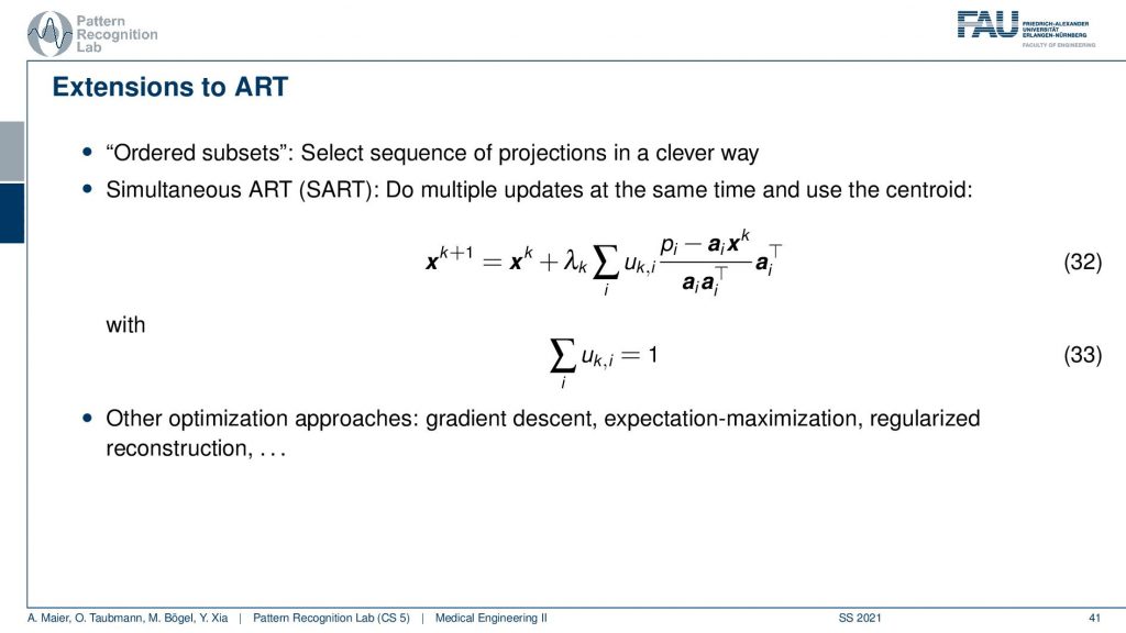
This can then also be constructed into an algorithm that is called the Simultaneous ART and there’s also variance in the ordered subsets. So ordered subsets are essentially skipping over projections. So let’s say you have your acquisition plane and then you have projections one, two, three, and four. Then what you would like to do is you want to use two and four because they’re orthogonal to each other. Then you update in the next steps one and three because they are orthogonal to each other. So you try to find projections that will help in the speed of convergence. So this is called ordered subsets and then there is also the Simultaneous ART where you essentially run updates over a kind of parallel processing. So you do multiple updates at a time and then average them. So this can also help you with increasing the conversion speed. There are many many more approaches we actually have a very nice lecture that is called Diagnostic Medical Image Processing where we go into all of these details and derive the methods and so on. For the time being, I think this is enough about iterative reconstruction. 

One thing that we still should discuss is the acquisition geometries. 

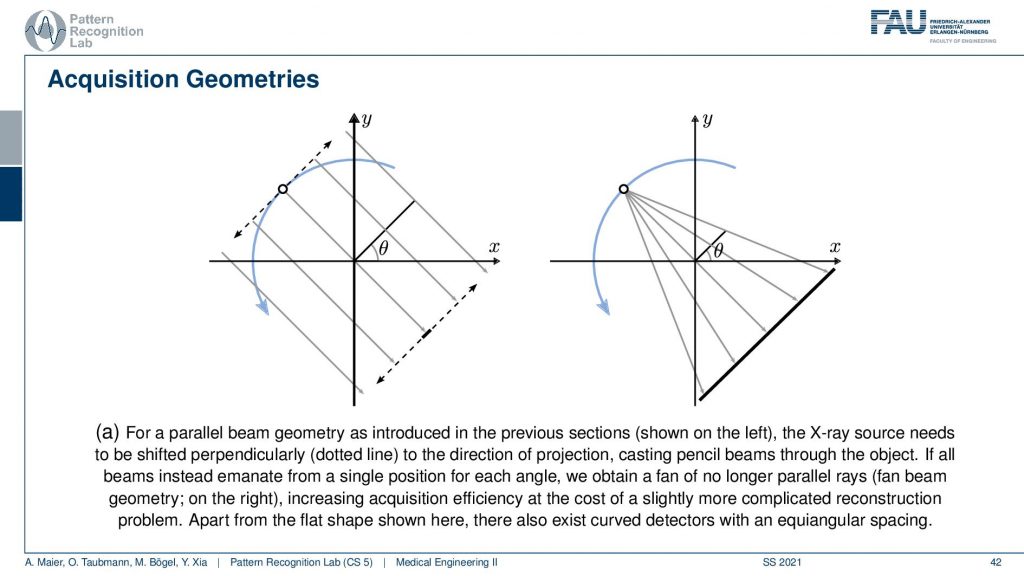
We’ve seen that the original Hounsfield scanner had this problem that we had to shift and the source as well as the detector element. Then we had to rotate and obviously, it’s much faster to work with just a single x resource and a linear detector because you can acquire all of these line integrals in a single shot. The problem with this is that you don’t have parallel geometry anymore. But the cool thing is that if you acquire a full circle, you have to rotate really by 360 degrees. Then you will see that from the other positions, let’s say this is the next position. Then you will of course also get additional line integrals here and here. If you look closely you will find that there is at least one ray in every new projection that is then parallel to another one. This way you can reorder the rays such that you get a parallel acquisition. So this kind of acquisition can be used for reordering and then you have a parallel geometry again. There are also direct solution methods that we have in diagnostic medical image processing. So this is much faster and then there is another trick.

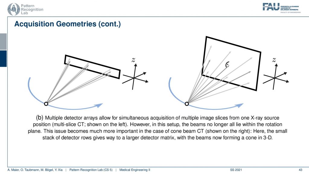
The next trick is that you don’t just acquire a single line detector but you start acquiring entire planes and you can make these planes as big as this. Then you start getting oblique rays. So they are not just within one plane but you really get a kind of pyramid. If you had a round detector this would be a cone. So this guy here is called cone-beam acquisition and this is even faster. But now you have the problem that some holes are appearing if you want to reconstruct the entire volume. This can be formalized in the so-called twist condition also something that we talk about in diagnostic medical image processing and this is incomplete. If you just acquire a circular scan but you want to reconstruct a complete cube here then you will not be able to observe all of the data by just rotating the wrong one here. This is where the headaches come in. So if you had a helix then you would acquire complete data. I’m not going through the proofs here but just to make sure by the helix or the shift and rotate kind of acquisitions are so important. 

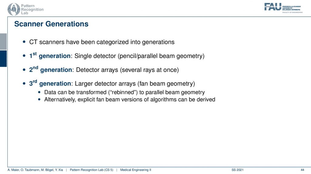
This brings us to different generations of X-ray scanners. So the first generation had a single detector and they had this pencil parallel beam geometry. The second generation had detector arrays and the third generation then had larger detector arrays with a complete fan-beam geometry. You will be using this re-binning trick in order to acquire larger portions at once and we also have other reconstruction algorithms for that.

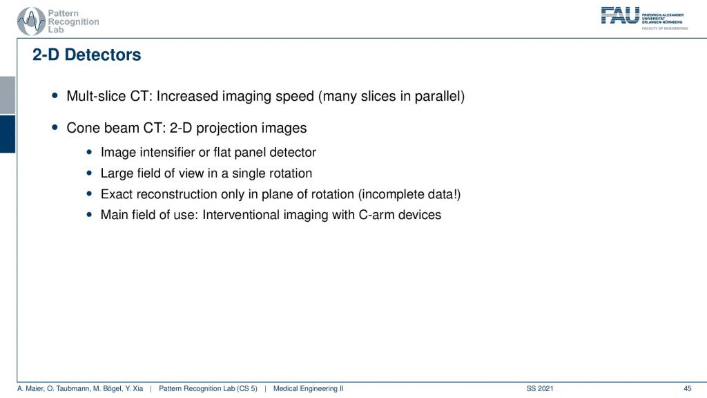
This then goes to 2D detectors and this leads us to multi-slice CT and cone-beam CT where we have this special geometry that follows this cone and this has, of course, a couple of mathematical challenges. But it can also be solved robustly which gives then rise to algorithms like the Feldkamp-Davis-Kress algorithm and they can then reconstruct the entire volume from a complete trajectory that is in living in a 3D space. One very popular example is of course the helical trajectory also. What’s pretty cool is that you can then also work with flat-panel detectors.

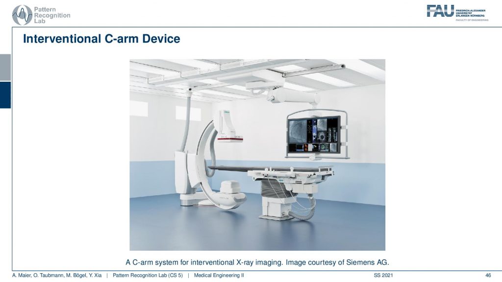
You see this is one of these angiography systems that were mainly built for doing fluoroscopy.  Because we now have the mathematics to solve also combine acquisitions we can also compute 3D images in the operation room. So you essentially take the system and rotate it about this axis here and then you have a CT acquisition. Then you can reconstruct entire volumes directly at the place of surgery and that’s really cool for neurosurgery. Then you can really get 3D reconstructions of the vessel tree of the patient on the table in close to real-time. So it takes about 5 to 20 seconds to perform such a scan and then you have a complete 3D volume. So this is pretty cool! 

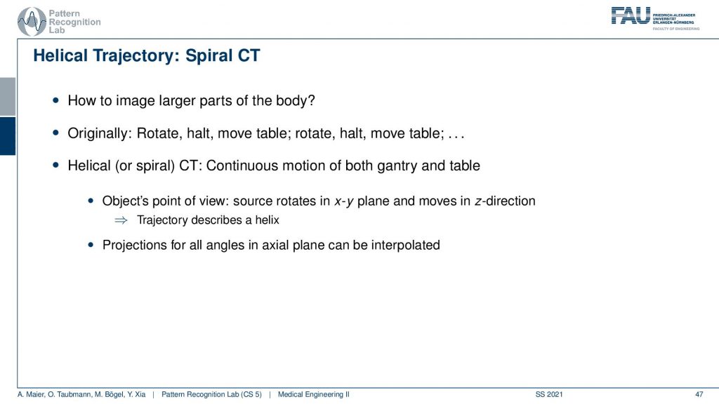
Well then the famous helical CT is that you now start moving the patient. So if this is the gantry and you have the patient and the patient is lying here. So you start moving the patient through the gantry at an appropriately z speed and this allows us to reconstruct all of the points of the patient at once and it is a complete trajectory. So this gives then rise to trajectories that look like this. 

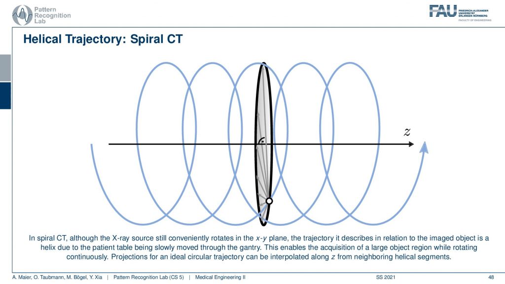
So you can think of the actual source position with respect to the patient is actually moving on this helix here. Because we’re moving the patient with respect to the source and this gives us this kind of helical or you could also say spiral motion in order to acquire everything at once. This is really complete and you can reconstruct without larger artifacts or missing data the entire 3D volume of a whole-body scan. So that’s really cool technology. 

Well, this already brings us to the end of this video. So you’ve seen here now the two main approaches for image reconstruction that is the filter back projection (a Radon inverse type) and also the algebraic approaches. The main difference between the two is the point in time where you discretize. So for the filtered back projection, you stay in the continuous domain as long as possible and discretize at the end. For the algebraic approaches you discretize right in the beginning; you immediately use voxel and pixel grids and then find the solution. You find two different solutions. One is iterative and the other one is directly computing the complete inverse. So I hope you liked this little video and some introduction to CT reconstruction algorithms. There’s more theory in the book that you can read and of course, we have this additional course that is called Diagnostical Medical Image Processing where we go into all of the details. But for the time being this is enough for us. In the next video, we want to discuss a little bit the difficulties that emerge in these kinds of settings. And this then leads us to the questions of spatial resolution noise and artifacts and images which we’ll discuss in the next video. Thank you very much for watching. Bye-bye!!

If you liked this post, you can find more essays here, more educational material on Machine Learning here, or have a look at our Deep Learning Lecture. I would also appreciate a follow on YouTube, Twitter, Facebook, or LinkedIn in case you want to be informed about more essays, videos, and research in the future. This article is released under the Creative Commons 4.0 Attribution License and can be reprinted and modified if referenced. If you are interested in generating transcripts from video lectures try AutoBlog

References   

• Maier, A., Steidl, S., Christlein, V., Hornegger, J. Medical Imaging Systems – An Introductory Guide, Springer, Cham, 2018, ISBN 978-3-319-96520-8, Open Access at Springer Link

Video References

1. Randy Dickerson – Syngo Via VB20 Cinematic Rendering https://youtu.be/I12PMiX5h3E
2. Tomographic reconstruction by Filtered Back-Projection https://youtu.be/-SiVPCh92TA

Category: Lecture Notes in Medical Engineering