Computed Tomography – Resolution, Noise & Artifacts

These are the lecture notes for FAU’s YouTube Lecture “Medical Engineering“. This is a full transcript of the lecture video & matching slides. We hope, you enjoy this as much as the videos. Of course, this transcript was created with deep learning techniques largely automatically and only minor manual modifications were performed. Try it yourself! If you spot mistakes, please let us know!

Welcome back to Medical Engineering. So today we start with the third part of CT and in this video, we want to look into spatial resolution, noise, and artifacts emerging in these images. You will get a better understanding of how the different sources affect the actual image quality that is produced at the end of the scanning choice. 

So part three of CT and we are now looking into the spatial resolution noise and artifacts. Now so far we have had theory and principles of CT and how to reconstruct the images. 

Now we want to look into the practical applications like how should the resolution of the system be, how will be different noise properties, and also how will artifacts look like. So these are essentially going deeply into the design aspects of the system that you have to consider actually before you actually build the system. So we’ve already seen that with the X-ray detectors that we have to know for example the design energies and so on because that is driving the decision for specific materials in the detectors. The same thing is of course also true when you’re designing a CT system for specific resolutions. 

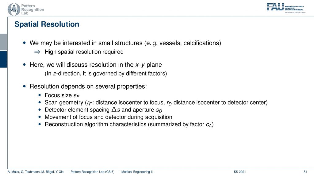
Spatial resolution is key for designing a scanner because we may be interested in structures of a certain size. You want to be able to see essentially vessels or calcifications and they may be pretty small. So we might want to have a high spatial resolution. So what we’ll discuss in the following is the resolution in the x-y plane and in the z-direction we won’t discuss this in too much detail. But we can only hint you at further courses like Diagnostic Medical Image Processing where also such ideas are discussed. So essentially this whole resolution of the system depends on all of its parts. So you see that the focus size plays a role. So this is s_F here, the scan geometry which is the distance to the focus from the isocenter and also the distance from the isocenter to the detector center. So the isocenter is the sensor of rotation right. Then also the detector element size and spacing essentially tells us how large the detector is and also how fine the pixel elements are. Also, the movement of focus and detector during the acquisition whether it’s a continuous motion and whatever this whole system has essentially is pulsed. So you just have a single X-ray pulse at a time and you get very sharp images. If you have a moving X-ray sourcing detector then also the motion will introduce a certain blur. Then of course the reconstruction algorithm also can emphasize certain characteristics of the system and this is now an additional factor here.

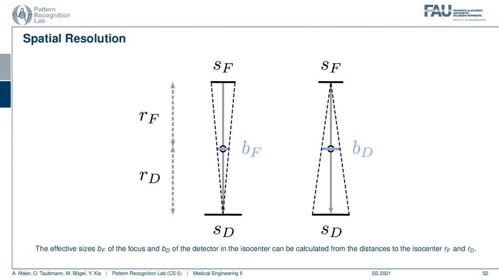
If we know about these things we can essentially determine the influence. You’ve already seen when we talked about the X-rays that of course, the size of the focus has a certain impact on the images. Now when we were talking about the X-ray projections we were interested on the projection of the focus into the image domain. But now it’s different because we’re rotating about our object. So this is the center of rotation and you can essentially see that you can determine a kind of a blur. So this is a blur of the focus and this is essentially the projection of the focus onto the detector. So this is the size in the X-ray tube and then it essentially gets scaled down towards the center of rotation. So this causes a blur. Now also the detector pixel size causes a blur and we essentially project it or scale it to the actual position in the isocenter. This gives us then b_D. So this is the blur introduced by the detector. Now we were interested in how to actually determine how this influences the reconstruction. Note that if you want to calculate this guy and this guy you have to be aware of the distances from the source to the detector and the isocenter. So these values have to be known and obviously also the source and detector size have to be known in order to calculate this. But this is very simple geometry. How to compute this now?

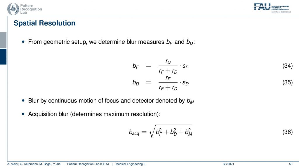
If you have that then you can also put this in equations. So we did that for you. So this is the source-detector distance and we have the distance isocenter and detector divided by the source-detector distance multiplied with the size of focus and this gives us the focal blur. For the detector pixels, it’s the very opposite. So it’s the detector pixel and here this is the isocenter to focus distance and this is divided by the distance from source to detector and this gives us the detective blur. Now if we have determined this then we can get the acquisition blur. This is the two blurs here squared and summed up. If you have a continuous source then there’s also some motion blur that is introduced because you essentially have the detector and the source moving about the patient and this is the third component. All of the three are then essentially squared added up and taken a square root and this gives you the acquisition blur. So this is a simple formula that can help you to determine the specific resolution of the system. 

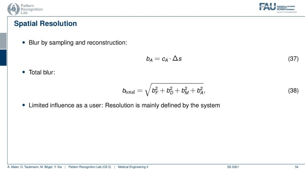
Now we can also expand this a little bit. We can also introduce the blur by sampling and reconstruction and therefore we need these two additional elements. This gives us then the blur of the acquisition and the total blur can then be estimated by adding this element here. So we see that we then determine the total blur and we already understand at this point that all of these parameters are essentially determined by the design of the system. So we can already predict very well what the resolution of the final system will be if we know how to deal with these parameters very accurately. 

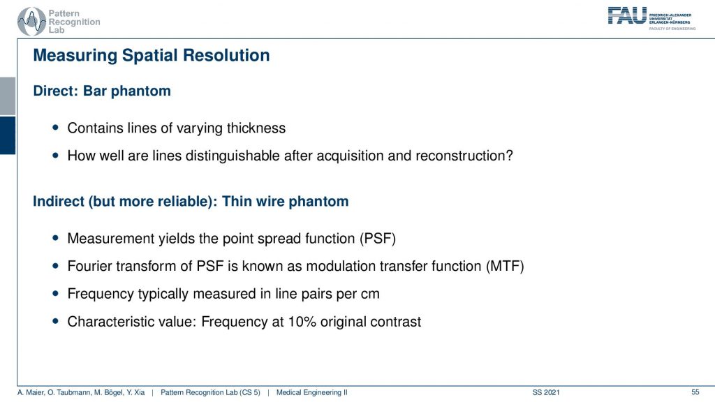
Now once we have built the system and you want to do all the considerations I just talked about before building the system. So this is our design specifications. Once you have built the system you want to figure out what is the resolution of the system. This can be done with a bar phantom or with a thin wire phantom and these are two approaches how to determine this and I will show them in the next couple of slides. So the bar phantom is essentially a sequence of black and white stripes that look like this in an intensity profile. If I have them at different frequencies you can see that when I take then images of these bar phantoms and I can resolve still this frequency but no longer this frequency, then I have determined the limit frequency. So this is the key idea behind that. The thin wire phantom works differently. So there you have essentially a Dirac pulse and then you send this into the system. You get a kind of blurred version of it and now you use the Fourier transform to determine the modulation transfer function. So you do the Fourier transform of this guy and this gives you the modulation transfer function. It can also be measured to figure out the actual resolution of the system. 

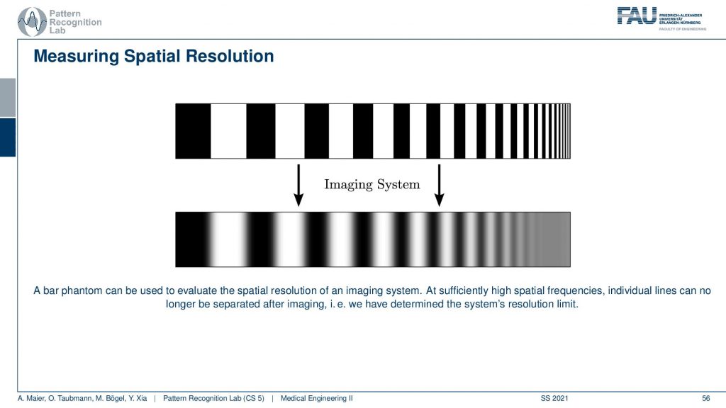
Let’s have a look at the bar phantom. So here you see that this kind of bar phantom starts with low frequency in the beginning and then it increases the frequency. So you could say we have an increase in frequency towards the end of this kind of bar stripe. So the period is reduced. So the wavelength of this kind of frequency is reduced to the right-hand side and then we apply the imaging system. So we essentially take a scan of it and then you observe something like this here. Here you can very neatly see that I can still observe all of those frequencies here. All of this is fine and then probably at this point here, I lose the resolution and now I have determined the limit frequency of the system. So here everything is gray and I don’t see any difference anymore and that’s the limit frequency of the system. You can also work with other patterns. So it’s not just these bar patterns. What you often find in photography is kind of wedges. So there you have essentially configurations like this one and then you paint those black. So in an alternating manner, you paint them black and if you do this you can already see what I’m constructing. I’m constructing essentially these pizza slices. The black pizza slices can also be measured as a kind of measure frequency and resolution. So you can now see that if I have concentric circles then they encode different frequencies. What’s also nice about this is if I now have a blur that is happening in a certain direction. So let’s say I’m blurring more in this direction. Then I can determine other limit frequencies in x and y of such a pattern and you sometimes see these kinds of patterns in photography. So these are actually constructed in order to determine the spatial resolution and the nice thing is this allows you to determine the resolution in x and in the y-direction. So that’s a pretty nice approach of how we can also use something similar to such a bar pattern but in two dimensions at the same time. Well, this is one approach. 

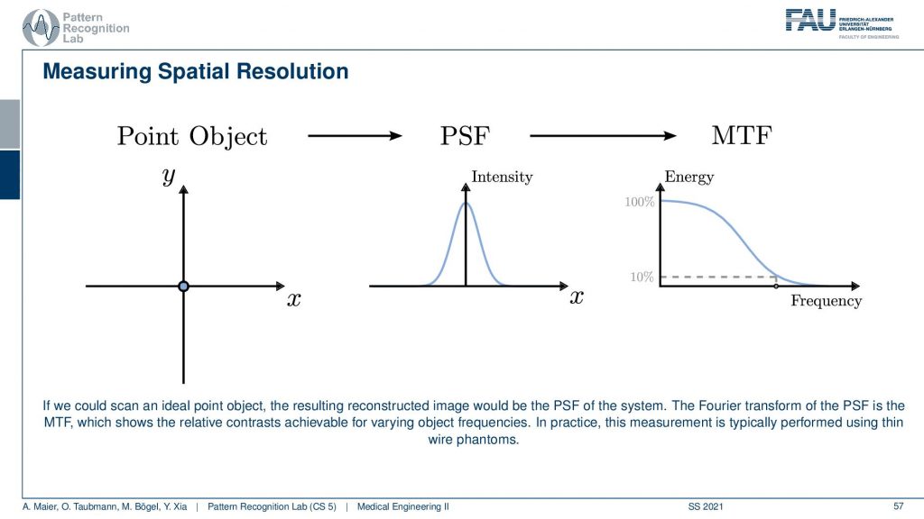
Another maybe a little more elegant approach is using a point object. So there you just have this point object that is finer than the resolution of the system. Then you image it and what you get is after measuring the response. You can see that this response here is a kind of Gaussian curve and this describes how well the different frequencies can be measured. Because if you remember the Fourier transform of a single direct pulse if you convert this to Fourier space the single direct pulse contains all of the frequencies. So this is the ideal kind of input. Now if I go ahead and measure then the Dirac pulse will essentially result in the so-called modulation transfer function and you can see it here. So this is essentially element-wise then multiplied with the characteristic of the system. You see that it typically has the shape as you see also in this image above here. Now you scale it and you scale it in a way that the maximum value is at 100% and now you can determine the limit frequency of the system as 10% MTF. So you could say okay everything here has so little contribution. That’s probably not visible. So now I do a very small measurement and it describes me essentially the entire characteristic of the system all because we’re using a Dirac pulse. By the way, his point object also measures the resolution in the x and y direction at the same time. One problem with those point objects is that the measurements are sometimes very noisy. So an alternative to this point object is the so-called slant edge measurement and there you’re measuring essentially an image that contains such a slanted bar and this bar is then black. So this is using the edge to measure. Now you take an image and you extract profiles all of those profiles here and now you can measure the average over all of those profiles. The nice thing is obviously you have to know the orientation of the edge but then you can average over all of those profiles and then you get a very nice kind of edge. The problem with this is this is not directly the point spread function and it’s only in the x-direction in this case. But obviously, this is nothing else than the integration over the point spread function. So if we now want to go from this edge profile to the original point spread function all I need to do is I need to compute the derivative with respect to the x-direction and then I’m back with the point spread function. This is typically much smoother and doesn’t suffer from noise as much as a single-point measurement. So these are typical approaches how to measure the resolution. The point object here sometimes in the industry this is also called the fast wire test. So you could take essentially the image of an wire. Then you place a slice in a way that it’s orthogonal to the wire direction and that is a very quick way that allows you to determine the image characteristics and the resolution characteristics of an object.

So now we know how to determine the resolution and we can now also talk about the noise. 

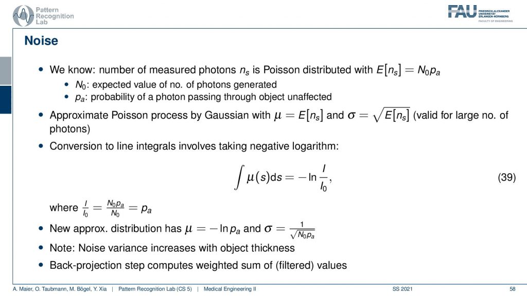
You remember when we were talking about X-rays we’ve seen that the noise is dependent essentially on the number of photons that arrive at the pixel. So we’ve computed that already in our video on X-rays. We’ve seen that the noise is essentially proportional to the square root of the number of photons that arrived at the respective pixel. So we can essentially determine this then from the measurement and if we had enough measurements and noise-free measurement we would know the expected noise for that respective pixel. This can be done for example by measuring the same image several times and then averaging. Then you can compute a noise estimate from the statistics that you have observed. This brings us to the very strange situation that the noise and the reconstruction may not be uniform because it’s different from all angles. 

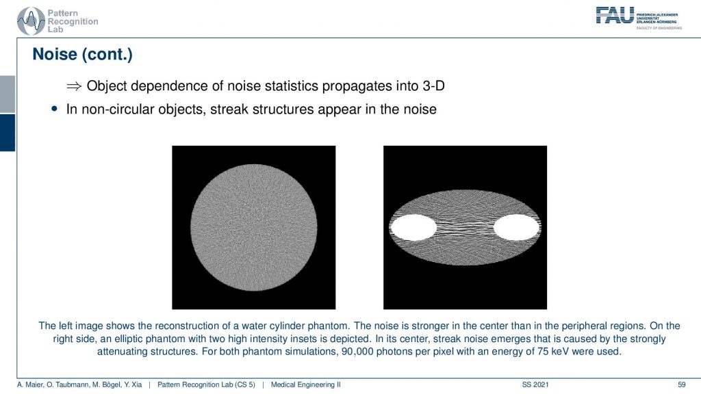
You can see that in the reconstructions in particular if you have a uniform object. So this is just a uniform water disk. What you observe here is that the noise is more pronounced in the center than in the outside. So there is less noise. So you have an increase of noise towards the center and the other effect that you can observe is that the noise may be streaky. Because if you follow this ray direction you see that there is a lot of material here on the beam in particular because I have this kind of bone structures in here. This then causes a certain noise to appear that has this streaky pattern. It’s just because from those views the noise contribution is much higher and although that we have a homogeneous material in between the two bones. There appears this kind of pattern and this is an artifact. This is caused by the reconstruction algorithm. It’s not there but it’s attributed to the different noise statistics. Just because there’s much more material here on this beam than on this beam, the noise variance in the two directions is very different. This causes then the emergence of these kinds of streaky patterns in the image. So this is also something that we have to live with and of course, there are also compensation methods that then also attribute the likelihood of noise being present in that certain pixel. We can compute that of course and then we can also consider that in the reconstruction algorithm in order to prevent these noise-like structures. 

This brings us to the topic of artifacts and there are tons of artifacts in CT images. The most important artifacts are beam hardening, scatter, partial volume effect, metal artifacts, motion artifacts, and truncation artifacts. We will discuss them in the following slides just to get an idea what is the cause of the artifact and maybe some idea how it could be compensated. What I find much more important is that you have seen them that you have a kind of catalog of artifacts and if you see them in the CT slice then you can maybe go back to this set of slides and say hey I’ve seen this artifact before. This is the reason this is causing our artifact. 

So this is also what a very experienced CT researcher will immediately see. He looks at the image and says okay this is this in this problem. So the experienced CT researcher has already a kind of catalog in the back of his mind. He can look at an artifact and say okay this is geometric alignment or, many of those different problems like motion and so on. He can immediately spot it just by the appearance of the artifact. So this is really something that has a lot of practical use that you understand where the artifact is actually coming from. Beam hardening is related to the energy dependence of our absorption coefficients. So you remember that if I sketch this very coarsely that if I have an X-ray spectrum I have a distribution like this right. So then I have a few characteristics and so on. So I have a distribution of different energies that are emerging and what then happens is if you go through the object and there is a lot of dense material, then the portion of low energetic photons will slowly disappear. What happens is that the more energetic photons are more likely to survive. This then effectively means that the average intensity of your spectrum moves to the higher energies and this is called beam hardening. So the more material you pass the more likely it is that the low energetic photons disappear and this causes a hardening of the beam. So this effect then causes the absorption to be not linear over the material length. So if I have let’s say a length of water or, some other bony structure or whatever material I have and then I have the absorption or not just the absorption, What will happen is that the actual length in the object which is the true path length and then this is the observed path length. So this is what I see from my photon statistics. Then I will see that I’m observing too many photons than I would expect. So there are too many photons surviving because the beam gets harder and has on effective higher energy. This will cause a mismatch between the true path length and the path length that we will measure. So what will happen is that I get an effect like this. So I kind of overestimate the path length. So obviously this goes to zero but we have a slant in this direction. So I think that more material is on the beam then is present because I lost many of the low energetic photons first. This appears then to be thicker than it is. 

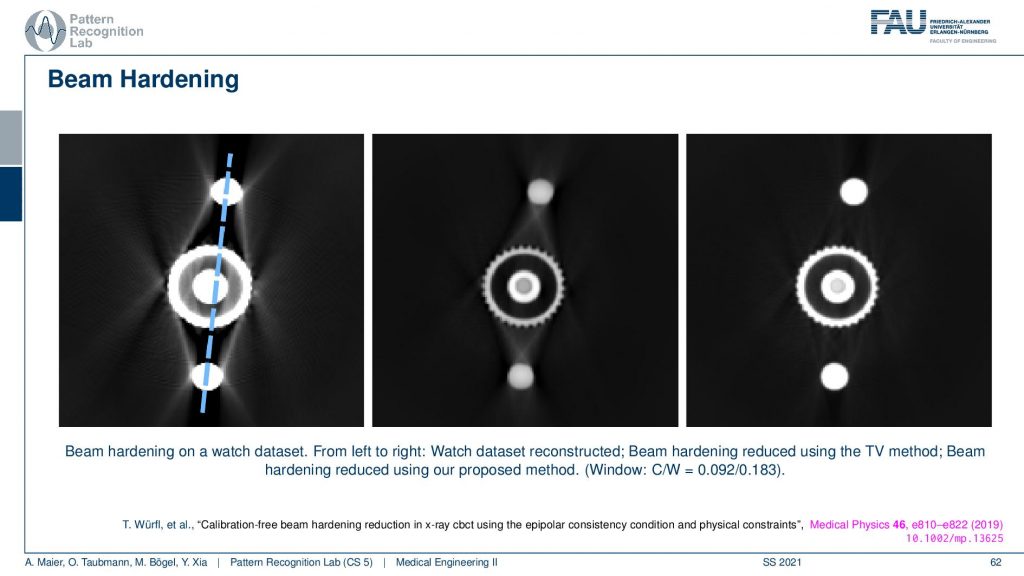
So this is the effect of beam hardening and you see typically as streaks in the reconstruction. You see here these typical streaks and they typically also appear in rays that have a long length of material of the hard material that it runs through. So you see that here these are rays that have a very long path length through the hard material and the same is here and here. So you get these connective rays that have this then excessive material that is spread along this ray. You see here a total variation base reduction algorithm and an improved consistency-based reduction algorithm. By the way, the reference is given down here. So this is worked by Tobias and colleagues. You can see if you model the physics correctly you can get rid of these artifacts quite well. But you have to estimate the non-linear effect that is disturbing your line integrals. So obviously in all of our reconstruction theory, we modeled everything to be linear and were just linear equations. But it’s not true. But if you model the non-linearity in a correct way you can get rid of these artifacts. 

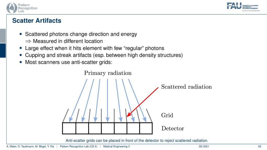
Well, there’s more to that there is so-called scatter. We’ve already seen that when our X-rays pass through the object they should be running like this. But then there is a scatter event and they change the direction and then there might be another scattering the event and then they get detected here. So what happens is that we essentially measure completely wrong signals here. So this has a longer path length and it also has the wrong intensity and so on. So it doesn’t convey the information that we want to have. In order to prevent these scattered photons from being counted what is quite frequently introduced is these lamellae here. And these lamellae are called anti-scatter grids. You will see they have also quite an importance in nuclear imaging. Their similar ideas are used and the idea of using these lamellae is that they are oriented towards the focal spot. Only rays that come exactly from the focal spot will hit the detector. While if you have a ray that gets scattered here and then counted here is going to hit the lamella at some point such that it will not be counted by our detector. So this is called an anti-scatter grid. The problem with the anti-scatter grid is that it takes away some of the intensity that is then not used in the image formation and it happens after the scattering event. So this is maybe not the best solution. But it’s one solution that helps you with getting rid of scatter. There are of course also algorithmic approaches that can help reducing scatter.

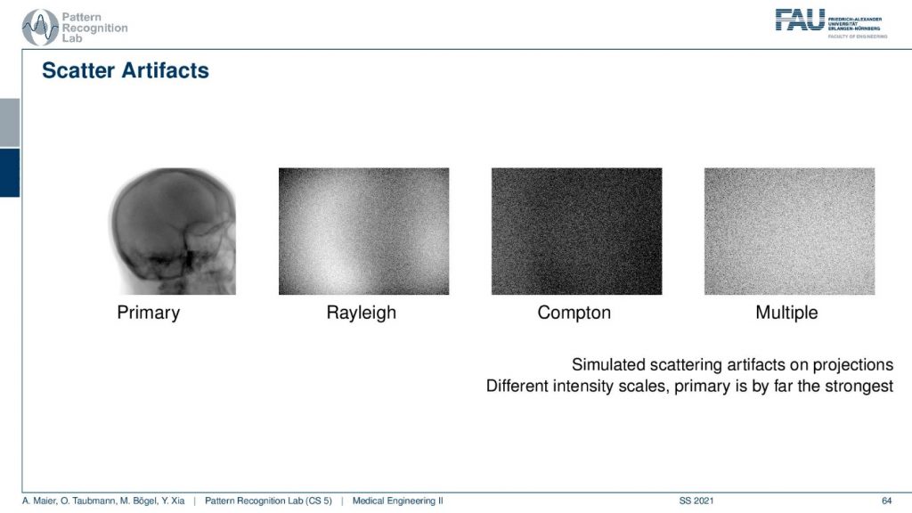
You will see that if you look at the scattering image domain so I have an example here. This is what you want to see. This is the primary signal. We can obtain this either with measurement or simulation where we really simulate the scatter events or you do a slit-scan and other techniques. So you can measure the direct radiation and this is what you would like to get. Now if I have a Monte Carlo framework where I simulate every photon I can even distinguish the different types of scatters. So the Compton and the Rayleigh scatter I can do that and then you see what the shape of the Rayleigh and Compton scatter is. Finally what I observe on the detector is the sum of the primary plus the scattered signals and here we even have multi-scatter. So this is a kind of scatter that has undergone several scatter events. Therefore I cannot separate it anymore to either Rayleigh or, Compton because you could also have mixed scatter events. So this is how the scatter masks then look like and what we measure at the detector is essentially the sum over all of those images. Of course, there are also scatter correction methods. 

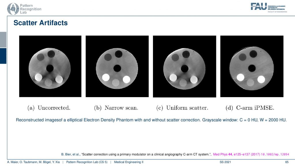
If you do not correct for scatter you get essentially images as you see here on the left-hand side. You see that this is supposed to look like this. So you see this is a disc phantom and there are different insets. What appears are these black stripes in between you get this unsharpness. You get artifacts here all over the place because the scatter contains information that is actually not correct in terms of geometry and therefore it causes a distortion of the geometry. What’s also very common in a homogeneous kind of phantom you would observe scatter often as this kind of cupping. So instead of reconstructing a straight profile, the influence of scatter causes your line profile. So if this is the disc phantom so this is the x and y and then you draw a line profile and you plot the intensities along this line. What you would like to have is an intersection like this. So this is all water but instead, you get this reduction towards the center. This is a typical scatter kind of artifact and then you can compensate it with different approaches. What we have here is a uniform scatter approach and then an iterative method here where we use a primary modulator that is able to measure and reconstruct the image at the same time. Here you see that the kind of artifacts is greatly reduced. So this image here is very similar to the image here. So you get rid of many of these stripes here. They don’t appear here. There are a few problems here on the outskirt. But you can see that this is already related to the acquisition here. So we had this artifact already here. So this is not a scatter artifact. But the scatter-based artifacts can be removed very efficiently with this kind of method. Again this is a paper that has been published here in medical physics. And this is a method by Bastian Bier et al. If you want to understand how the method works you can readily download the paper.

What other effects appear?

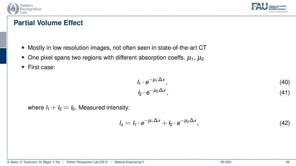
 There’s also something that’s called the partial volume effect. It is essentially considering what’s happening within one pixel because there might be several materials in one pixel. So there could be a material μ₁ and a material μ₂ in the same pixel. If you would observe them then you would independently get the I₁ times the material μ₁ and some I₂ times the material μ₂. Then you would like to get the total absorption and the total absorption here would be I_x which is the sum of the two absorptions. Now, this is what would happen in this case if you model them distinctly. 

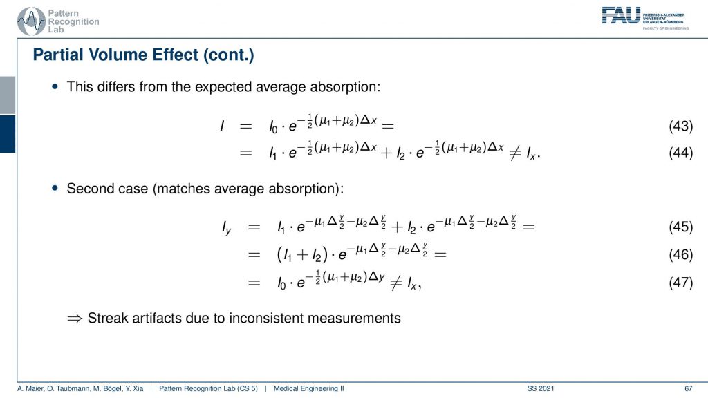
Now what we typically do in a reconstruction algorithm is we model them as a combination as a linear combination of the two in the same voxel. So you get something like μ₁ plus μ₂ divided by two. So the average of the two is given that they have the same proportion in the same pixel. If you then do the math and calculate this, then you see that this is not the same as I_x. So even if you model this as average absorption you won’t get this equal to I_x. The mismatch between these two configurations modeling this as a sum in the pixel and independent path lengths along the ray you see that we never get the same result and this then causes streak artifacts due to the inconsistent measurements. So we have some examples of this here.

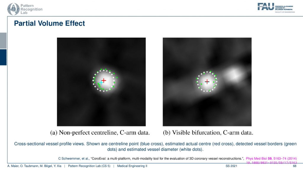
What is also very common for the partial volume effect is that if you have a wire so this is supposed to be a very sharp object that is uniform. If you look through a plot here you will see what happens is that you don’t get something like this that there’s a material of clear boundaries but instead you’re measuring something like a kind of blooming artifact. The big problem with this is depending on what kind of threshold you pick. So let’s say I take this intensity threshold or this intensity threshold and then I want to measure the diameter. You see if I take the lower one or if I take the higher one then I may be ending up measuring very different diameters. So this is a huge problem in measuring for example vessel diameters in CT volumes. If the resolution of the grid is not fine enough because then you get these tons of problems. Measuring the quality of vessels is an art of its own. My colleague Chris Schwemmer has a very nice paper on how to evaluate the quality of different vessel depictions and he had a small software framework to put these things together. 

There are also metal artifacts. Now metal artifacts are even worse than beam hardening because what can happen is that first of all the metal typically has very different absorption characteristics than the water that is typically present. So there’s a huge fraction of beam hardening that occurs with metal. But what can also happen is that you have so strong attenuation that there is not a single photon arriving on the detector. This is bad because we are computing this minus ln of I over I₀ and now that is zero. So you’re taking the logarithm of zero and then the minus if you remember how the shape of the logarithm is you remember that it has this kind of shape. So you’re going towards minus infinity. So if you haven’t observed if you flip it with the minus then it’s going to be plus infinity. So if you don’t observe a single photon your observation will be that there is an infinite thickness along the path. This is bad because you know you’re doing line integrals and suddenly we have infinity in there. This will cause a lot of problems. So typically you then assign a maximum value for this ray. But still, the ray will cause significant streaks in the reconstruction, and of course, there are some ways how to mitigate this. So you can increase the tube current because then you have a better contrast in metal. You have metal artifact reduction algorithms and they try to remove the metal objects in the projection and then replace them with the best knowledge that we have about the object. This can also help to reduce the streaks. Here you see an example. 

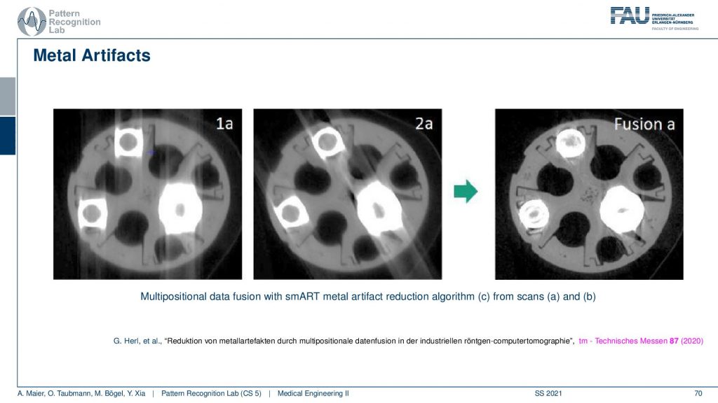
So this is using different positioning. We’ve already seen that the longer the path through the metal is the stronger the artifact is. You see here that these are two scans and in one scan the direction of the beams follow here. So you see the pronounced artifacts in this direction. In another scan, you see that the direction of the beams is following this direction. So you see that the rotation planes are not directly around the slice but in an orthogonal view. You can vary in 3d the plane of rotation. If you do that for two different setups let’s say this might be a rotation in this direction. Then you take this guy and this guy and you adjust according to the path lengths. So you essentially assign different amounts of trust to every observation and this allows you to reconstruct then a much better-resolved image. Here you can see the metal very well. But if you do stuff like this you have to do two scans. So this may not be that great after all. There are also very clever path planning techniques by colleagues at Johns Hopkins for example Matthias who would design methods that then automatically adjust the scanning path(the scan trajectory) such that you get minimized metal path lengths in order to mitigate metal artifacts.

There is at least one more that I want to talk about and this is the so-called motion artifact.

This is related to non-static objects and happens all the time. I mean if you have a scanner that’s fast enough for scanning like the dual-source system like the flash this is a good system for scanning the heart. But if you just have a classical scanner or even an interventional scanner that takes like 5 to 20 seconds for the rotation, you will have motion artifacts. This causes either blurring or, streak or, effects and in particular, in the interventional systems, it happens all the time. In order to alleviate that problem, you have to estimate the motion that was happening in the scan and then you deform the object in such a way that it is virtually frozen and this then allows volumetric reconstruction. So I have an example here of what can be done and this is using markers.

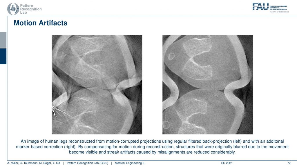
So we attach markers this is a scan of the knee. This is what came out of the scanner without motion compensation. It’s a person standing and you see here the kneecap and this is the knee bones. Yeah, but you can only observe this after the motion compensation. What we did is we attached essentially tiny metal beads on the leg of the patient and then we observed them in every X-ray projection. So once we go around we always see these kinds of metal beads right. From the position of these beads, we can estimate how the leg has been moving overtime throughout the acquisition. Because we know that the beads are attached to the leg. So if I move them into a coordinate system where they’re always in the same position, I have a virtually frozen leg. Then I apply this motion during the back projection in the reconstruction formula and then I get the right-hand image from the left-hand image. looks like magic doesn’t it? But it’s just mathematics and some considerations about the actual acquisition process. very well!

There is one more artifact that I want to talk about and this is the so-called truncation artifacts. 

This happens if you’re imaging a patient that is larger than your field of view. Let’s say you have this detector and this is your patient. So you see then we suddenly don’t observe the entire profile. The problem here is that this is essentially equivalent to observing the patient like this. Then we are multiplying with a one zero function that is the size of the detector and then what we measure is a function that maybe looks like this one. So we still have the roundness in this kind of interval but all the other information here all this stuff is lost. We never acquired this and that’s a problem because then the line integrals don’t add up anymore. We are essentially missing the mass here. So we’re missing the mass here and our line integrals don’t match up anymore. So the reconstruction doesn’t make sense. It can be solved. So there is theoretical evidence or proof that you can also reconstruct the inner part. So if this is the actual patient and you acquired still a 360-degree scan then you will be able to reconstruct essentially the intersection of all the cones that have been used to scan the patient. If it’s a rotation then you typically end up with a circular area inside the patient that can be reconstructed. But it can only be reconstructed up to an offset because we never essentially see how large the patient is. We don’t know what’s the patient this size or was the patient actually this size but a little denser. So we can’t differentiate whether the patient was slimmer and dense or bigger and less dense. This is what we can’t tell from the interior problem. This then essentially gives us that the reconstructions can be up to a scalar factor s. This is what we are missing. So this is one thing if you’re working with filter back-projection type of algorithms. You will see that multiplying with such a step function maybe not be such a great idea. Because you’re essentially convolving with the Fourier transform of this in Fourier space. This then causes a pretty heavy artifact. So we see that on the next slide here.

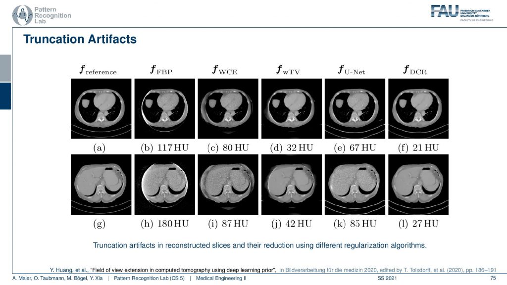
There we show different truncation correction approaches. So this is the complete scan, this is the reference. So this is two different sections and you see here essentially that these are two sections and you could say that this is our patient right. One section is more through the liver and the abdomen and the other is through the heart. So this is the heart and the lungs and this is the abdomen showing the liver and other organs. Now if you do truncation what happens is you’re missing stuff. You’re missing the stuff here and you’re missing the stuff here. What you can do is you can do a water cylinder extrapolation. So this is a very simple approach. We say okay everywhere outside the field of view the patient just behaves like a water cylinder. Then you can get reconstruction results like this. So we just make up something that may be plausible or not and what you see is the key artifact that is reconstructable. But you see this white stripe and all of these artifacts are gone after the body cylinder extrapolation. But obviously, the stuff outside the field of view doesn’t make any sense. So this is not good. Then you can of course use a different kinds of reconstruction algorithms. You can use a kind of Tv approach. So this is minimizing the total variation. It’s an iterative method slightly better and gets within the field of view. It gets a pretty good error but it doesn’t complete the image very well. There is stuff from deep learning. So we can just use a deep network and artificial intelligence to predict what’s probably outside and this is fairly good. This does a fairly good job in completing those areas here. If you look at those they’re very similar to our reference. But they just make up stuff and this results then in a larger era within our field of view. So this is the part that we can reconstruct and because we do errors in the extrapolation it also increases the error within the field of view. Yeah and then you can mix the two so you can initialize with a kind of deep learning approach and then you essentially get the best of both worlds. So you get a very good reconstruction error inside the field of view and you still get a plausible completion here towards the outside. So these images now may be very small. So if you want to study them in more detail you can either go to this conference paper here or download the slides from our online resources and then you can also have a look here. So that’s a pretty cool result. very well!

So this already brings us to the end of this video. Now we discussed the actual acquisition and the theory of how we can make projections, come together as slice images again. We looked into the actual reconstruction algorithm. So we had the analytical ones, the filtered back-projection type of methods as well as the iterative ones that are pursuing an analytical discrete solution. Then we’ve seen the world of artifacts, noises, and resolution in this video here. There’s one more thing that I would like to show you about CT reconstruction. So there’s even a fourth video a kind of bonus video that we’ll talk about in the next session and this will discuss spectral CT. So we see this energy dependence that causes a lot of artifacts and in the next video, we want to discuss what happens if you model that correctly and what kind of opportunities we have if we get the physics modeled correctly into the reconstruction reference. Okay, so I hope you enjoyed this small video and I’m very much looking forward to seeing you in the next one. Bye-bye!!

If you liked this post, you can find more essays here, more educational material on Machine Learning here, or have a look at our Deep Learning Lecture. I would also appreciate a follow on YouTube, Twitter, Facebook, or LinkedIn in case you want to be informed about more essays, videos, and research in the future. This article is released under the Creative Commons 4.0 Attribution License and can be reprinted and modified if referenced. If you are interested in generating transcripts from video lectures try AutoBlog

References   

• Maier, A., Steidl, S., Christlein, V., Hornegger, J. Medical Imaging Systems – An Introductory Guide, Springer, Cham, 2018, ISBN 978-3-319-96520-8, Open Access at Springer Link

Video References

1. Fix it like a Boss – 4k TestPattern https://youtu.be/S7SLep244ss
2. C-Spine with Cinematic Rendering https://youtu.be/hEOf8g_I1-w
3. Siemens Artis Zeego Q in der Radiologie https://youtu.be/wjM69jQWJDw

Category: Lecture Notes in Medical Engineering